What to build

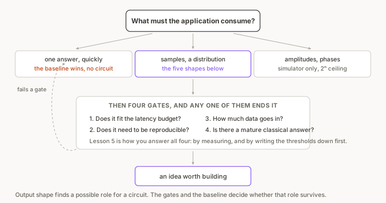
Choose a quantum project by the output your application needs. A circuit gives your program exactly one thing, a distribution over bitstrings, and every application built on one consumes that distribution in one of five ways. An idea that fits none of the five does not need a circuit. Picking a famous algorithm first and then looking for a place to use it often turns up nothing that fits.

Five things you can do with a distribution

Sample from it. You want draws, and you use the spread of outcomes directly. The picker you built takes this shape, and so does most generative work, where any given draw is as valid as another.

Quantum Garden maps five qubits' thirty-two outcomes to a plant's traits. Superposition Sequencer, by Francisco Estivallet, turns every note in a music sequencer into a draw from a circuit you designed. Quantum Patterns, by Peter Thomas and Paulo Itaboraí, uses partitioned quantum cellular automata to make musical material you can live-code against.

Compare two of them. You have a live state and a reference state, and you want a similarity score between them. Regime Radar prepares a fingerprint of current market conditions, runs a stored regime backwards over it, and reads the fraction of shots landing on all zeros as the overlap: when the two states match, the shots concentrate there.

Read structure inside it. You care less about which outcomes appear than about how the bits relate: which qubits agree, which are correlated, how that changes layer by layer. Butterfly Field turns pairwise entanglement into the threads between its butterflies. QCFlows renders the same structure as a live graph. Entangled Body, by Chanhyuk Park and Luke Shim, builds a point-cloud figure whose parts, per its write-up, respond to each other across distance.

Classical simulations of many entangled qubits get expensive quickly, so this shape has the least obvious classical shortcut.

Reduce it to one number. You want a score, and the distribution is only an intermediate. The Quantum Systemic Oracle reduces an optimization result to a single risk index. qOrbital, by Aryan Bawa and Arnav Singh, runs a chemistry calculation and reads out a molecule's energy. Quantum Market Game, by Aadarsh Venkat Ramanan, models two traders as two entangled qubits and reads their payoffs out of the tally.

Watch it change. This shape reads the statevector rather than a tally, so per lesson 2 it only exists on a simulator, which is enough for a tool that shows someone what a circuit is doing. QAVE, by Inho Choi, makes an algorithm visible gate by gate. Quantum Advantage Lab, by Hossein Sadeghi, streams four algorithms' intermediate state beside their classical counterparts. Quantum Canvas, by Shivani Mayekar, lets you drag operations into a circuit and watch the result move.

Watching it change is also the easiest of the five shapes to ship, because nothing queues.

Ideas that do not map

Most ideas do not map, for one of four reasons.

It needs one correct answer, quickly. A distribution is not an answer, and lesson 5 measured what the round trip costs. If your feature can be written with a lookup or a solver that returns in milliseconds, it should be.

It needs to process a lot of data. Getting classical data into a quantum state costs roughly one operation per number, so loading a large dataset takes longer than reading it. Your laptop already solves the problems small enough to fit on today's machines, and solves them exactly.

It needs the state itself, at scale. The fifth shape, watch it change, is fine for a teaching tool on a handful of qubits, but simulating n qubits takes 2ⁿ numbers, so an application built on statevectors hits a qubit limit quickly.

It needs to be reproducible. Two presses of an unchanged circuit disagree, as lesson 2's two Garden runs did. If your feature must produce the same output twice, the circuit has to sit behind a cache, which is the precomputed-pool shape from lesson 4.

These four reasons do not stop you learning, prototyping or building something because it interests you; they apply to shipping a feature.

The shape of a good first idea

The projects in this course share three things: a small circuit, a decode step doing most of the visible work, and a stated reason for the quantum part to be there.

Garden needed a supply of unpredictable, structured variation, and a pool of measurement outcomes gave it one. Butterfly Field set out to make entanglement visible. Regime Radar needed a similarity measure and chose a kernel that a circuit computes directly.

None of the three needed to beat a classical computer, which lesson 5 showed is rare today.

From one probability to two inputs and four named outcomes

A probability is the smallest thing you can put through a circuit. An application has several, and it needs its results named before anything can branch on them.

The next step up has two independent inputs, one qubit for each, and four named outcomes.

​# 'backend' already exists when this runs: it is whatever you pick in the Run Experiment dialog.
​from math import asin, sqrt
​from qiskit import QuantumCircuit
​from qiskit.providers.jobstatus import JobStatus
​import time
​​
​shots = 1000
1p_left = 0.2
2p_right = 0.8
​​
3NAMES = {
​    "00": "neither",
​    "01": "left_only",               #   key is c1 c0, so the RIGHT character is qubit 0
​    "10": "right_only",
​    "11": "both",
​}
​​
​​
4def build_circuit(pl, pr):
​    qc = QuantumCircuit(2, 2)
​    qc.ry(2 * asin(sqrt(pl)), 0)
​    qc.ry(2 * asin(sqrt(pr)), 1)
​    qc.measure([0, 1], [0, 1])
​    return qc
​​
​​
5def decode(counts, n):
​    return {NAMES[k]: v / n for k, v in sorted(counts.items())}
​​
​​
​job = backend.run(build_circuit(p_left, p_right), shots=shots)
​while job.status() not in (JobStatus.DONE, JobStatus.ERROR, JobStatus.CANCELLED):
​    time.sleep(5)
​​
​counts = job.result().get_counts()
​print(counts)
​​
​for name, share in sorted(decode(counts, shots).items()):
​    print(f"{name:11s} {share:.3f}   {'#' * int(40 * share)}")
​print(f"expected both = {p_left * p_right:.3f}, neither = {(1 - p_left) * (1 - p_right):.3f}")
1one input per qubit: how often the left step fires
2and the right one
3the result schema the rest of the app codes against
4two app values in, one two-qubit circuit out
5counts in, named results out

Three things changed from the picker, and all three are the parts you would write for any application.

Two inputs, two qubits. p_left and p_right each get their own ry. Nothing entangles the two qubits, so the four outcomes are the two probabilities multiplied out, and calling random.choices twice would do the same job.

A result schema. NAMES turns bitstrings into neither, left_only, right_only and both. The rest of the program branches on those words and never sees a bitstring. Adding a third input later means changing this table.

The bit order, stated once. A counts key reads c1 c0, so the rightmost character is qubit 0, and 01 means the left step fired and the right one did not. Get this backwards and your application does the opposite of what you meant, silently, because both keys are valid.

Our run on 22 September 2026, with p_left = 0.2 and p_right = 0.8:

{'00': 172, '01': 56, '10': 621, '11': 151}
both        0.151   ######
left_only   0.056   ##
neither     0.172   ######
right_only  0.621   ########################
expected both = 0.160, neither = 0.160

The ideal shares are 0.160, 0.040, 0.640 and 0.160. Every measured share sits near its ideal.

Takeaway

Start from what your application consumes and choose the algorithm last. Match the output to one of the five things a distribution can do, then check the idea against the four reasons ideas fail to map.