Project Showcase: qOrbital

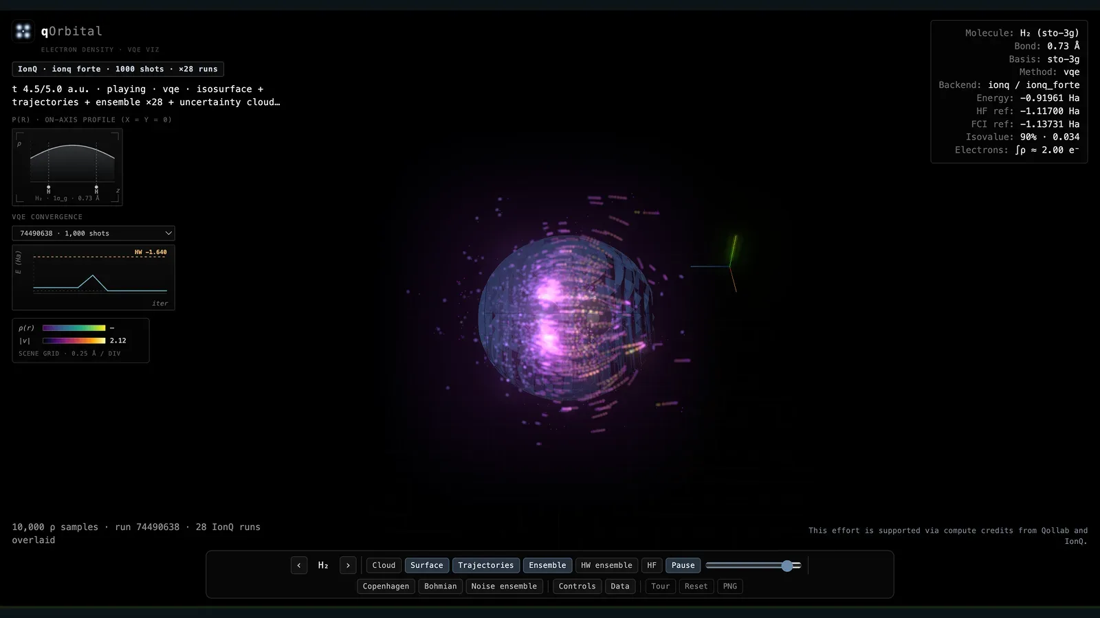
When a chemist draws a molecule, the electrons are not really dots. They are fuzzy clouds of probability. qOrbital computes those clouds for small molecules on real quantum hardware, then lets you look at them.

Pick a molecule (H₂, HeH⁺, LiH), drag a bond-length slider, and a full quantum-chemistry pipeline runs underneath: classical integrals from PySCF, a qubit Hamiltonian from Qiskit Nature, and a ground state found by VQE on IonQ. From that state qOrbital reconstructs the electron density and renders it. It is built by Aryan Bawa and Arnav Singh, two Dartmouth physics students, and its sharpest idea is what it refuses to hide.

Most VQE demos report one energy number and hide the noise. qOrbital makes the noise the exhibit.

Two ways to see an electron

What does an orbital actually look like? Quantum mechanics gives two famous answers, and qOrbital shows both from the same wavefunction. The Copenhagen view is the textbook one: a probability cloud, rendered as a 3D density isosurface. The Bohmian view takes that same wavefunction, computes a velocity field from its phase, and integrates particle trajectories through it.

Drop a handful of seed particles into the Bohmian view and they do not fill the orbital so much as draw it. Paths bend around nodes and crowd where the bonding density is highest. You set a molecule and a geometry, and the orbital responds in real time as you move the slider, with a live dashboard showing the VQE optimizer working its way toward the ground state.

Two radically different interpretations, one underlying wavefunction, side by side. The connection becomes something you watch instead of something you are told.

Noise you can see

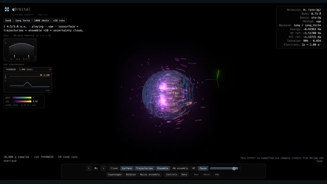
This is the part no other visualizer does. Bohmian trajectories need a high-fidelity wavefunction, not just an energy expectation value, so every hardware run carries the full fingerprint of finite measurement statistics. Overlay many independent IonQ runs and you get a trajectory uncertainty cloud.

Where the physics is robust, the trajectories pile up sharp and clean. Near nodes, where the wavefunction is most fragile, they smear out. The error stops being an abstract bar on a chart and becomes a shape you can read.

Instead of a dry error bar, you see exactly where a trapped-ion processor is and isn't sure.

To make that explorable without a hardware queue, real runs on IonQ Aria and Forte are bundled as a gallery of independent results per molecule, so visitors can browse genuine hardware output, run-to-run variation and all, while a clean Aer statevector simulator provides the "this is what perfect looks like" baseline.

How it works

The pipeline is a real quantum-chemistry stack, end to end: PySCF builds the classical integrals and a Hartree-Fock reference, Qiskit Nature maps the fermionic problem to qubits, VQE finds the ground state, and the optimized state is turned back into a density grid and a Bohmian velocity field for rendering. The core loop is small enough to run yourself, and on Qollab it runs as written:

# qOrbital quickstart: find a molecule's ground state with VQE.
import numpy as np
from qiskit.primitives import StatevectorEstimator
from qiskit_algorithms import VQE
from qiskit_algorithms.optimizers import SLSQP
from qiskit_nature.second_q.circuit.library import UCCSD, HartreeFock
from qiskit_nature.second_q.drivers import PySCFDriver
from qiskit_nature.second_q.mappers import JordanWignerMapper

MOLECULE, BOND = "H2", 0.735          # also: HeH+, LiH

# 1. Classical chemistry: Hartree-Fock + molecular integrals
problem = PySCFDriver(atom=f"H 0 0 0; H 0 0 {BOND}", basis="sto-3g").run()?Classical setup. PySCF runs Hartree-Fock and builds the molecular integrals. This is also the classical baseline qOrbital compares against.
# 2. Fermions to qubits
mapper = JordanWignerMapper()?Mapping. Turns the fermionic Hamiltonian into qubit operators. LiH instead uses parity mapping with a 2-qubit reduction to keep the qubit count down.qubit_op = mapper.map(problem.hamiltonian.second_q_op())

# 3. UCCSD trial state, from the Hartree-Fock reference
hf = HartreeFock(problem.num_spatial_orbitals, problem.num_particles, mapper)
ansatz = UCCSD(problem.num_spatial_orbitals, problem.num_particles, mapper, initial_state=hf)?Ansatz. UCCSD is the trial wavefunction. VQE tunes its parameters to push the energy down to the true ground state.
def show(step, params, energy, meta):
    print(f"  iter {step:>3}   E_elec = {energy:+.6f} Ha")?The descent. VQE walks downhill: each step the optimizer nudges the circuit and the energy drops. This callback feeds the live convergence dashboard.
vqe = VQE(StatevectorEstimator(), ansatz, SLSQP(maxiter=100),
          callback=show, initial_point=np.zeros(ansatz.num_parameters))
result = vqe.compute_minimum_eigenvalue(qubit_op)

total = result.eigenvalue.real + problem.hamiltonian.nuclear_repulsion_energy?Electronic energy plus nuclear repulsion is the molecule's ground-state energy. qOrbital rebuilds the electron density and Bohmian trajectories from this state.print(f"  ground state = {total:+.6f} Ha")

From the converged state, qOrbital extracts the one-particle reduced density matrix to rebuild the electron density on a 3D grid, computes the de Broglie-Bohm velocity field v = (ℏ/m) Im(∇ψ/ψ) and integrates it with adaptive Runge-Kutta for the trajectories, then renders both with Three.js on the web and PyVista in the lab.

Make it yours

qOrbital is open and forkable on Qollab, the full package is MIT-licensed on GitHub, and you can try the hosted demo right now. Swap the molecule, change the bond length, seed your own particles, and rerun the VQE on a simulator or real IonQ hardware. Supported molecules today are H₂ (the tutorial baseline), HeH⁺ (polar asymmetry), and LiH (the main showcase).