Is quantum worth it in your app
Run the same job both ways and compare the counts and the timings.

You answer whether quantum is worth it by measuring: race.py draws the picker's thousand samples twice, once with one line of ordinary Python and once with the circuit from lesson 3, and compares the two runs on count and on time.
The race
The file runs both methods once and scores them with the same arithmetic.
# 'backend' already exists when this runs: it is whatever you pick in the Run Experiment dialog.
from math import asin, sqrt
from qiskit import QuantumCircuit
from qiskit.providers.jobstatus import JobStatus
import random
import time
shots = 1000
p_rare = 0.3
# --- the conventional answer -------------------------------------------------
t0 = time.perf_counter()
1picks = random.choices(["common", "rare"], weights=[1 - p_rare, p_rare], k=shots)
classical = {"rare": picks.count("rare"), "common": picks.count("common")}
classical_s = time.perf_counter() - t0
# --- the quantum answer ------------------------------------------------------
qc = QuantumCircuit(1, 1)
2qc.ry(2 * asin(sqrt(p_rare)), 0)
qc.measure(0, 0)
t1 = time.perf_counter()
job = backend.run(qc, shots=shots)
while job.status() not in (JobStatus.DONE, JobStatus.ERROR, JobStatus.CANCELLED):
3 time.sleep(1)
counts = job.result().get_counts()
quantum = {"rare": counts.get("1", 0), "common": counts.get("0", 0)}
quantum_s = time.perf_counter() - t1
# --- read the result honestly ------------------------------------------------
print(f"classical {classical} in {classical_s * 1000:.2f} ms")
print(f"quantum {quantum} in {quantum_s:.1f} s")
print()
gap = abs(classical["rare"] - quantum["rare"])
print(f"the two draws differ by {gap} out of {shots}")
print("two independent 1,000-shot draws land within 40 of each other 95% of the time,")
4print("so anything up to about 40 here is the two methods agreeing.")
print()
print(f"the quantum run took about {quantum_s / classical_s:,.0f} times as long,")
print("almost all of it queue and round trip rather than computation.")
- 1the whole classical solution
- 2the same distribution, prepared as an amplitude
- 3poll every second, so the timing below has 1s resolution
- 4from the binomial, not from this run
The classical side is one call to random.choices with weights. The quantum side is the circuit from lesson 3. Both produce 1,000 draws at the same probability, and the file times each.
Open the project, press Run on Qollab, choose IonQ Aria 1 (25q) under Remotely Run Simulators, and press Run. Our run on 22 September 2026:
classical  {'rare': 281, 'common': 719}   in 0.20 ms
quantum    {'rare': 292, 'common': 708}   in 13.8 s

the two draws differ by 11 out of 1000
two independent 1,000-shot draws land within 40 of each other 95% of the time,
so anything up to about 40 here is the two methods agreeing.

the quantum run took about 69,044 times as long,
almost all of it queue and round trip rather than computation.
The two columns hold the same answer. Two samples of one distribution land within about 40 of each other at this many shots, and these are 11 apart, so neither column is more correct than the other.
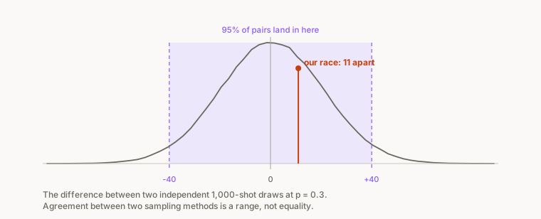
That 40 is the figure for p_rare = 0.3, and the listing prints it whatever probability you set. The true window is widest near 0.5, about 44, and shrinks toward zero as the probability moves toward 0 or 1.
The two timings differ by about 69,000 times, which no tuning of the circuit would change: nearly all of that time is the round trip to IonQ's cloud.
The quantum column came from a simulator
You ran on a simulator. The IonQ simulator is a program on a server, so the numbers in the quantum column were produced by classical hardware doing arithmetic, with no physical measurement involved.
So the race you just ran compares one classical method against another classical method that took 69,000 times longer. On real hardware the quantum column would come from a physical process. The timing gap would grow, because a QPU has a queue in front of it, and each run would cost credits.
A measured draw has no seed
On hardware, the draw comes from a measurement rather than from an algorithm. random.choices is a deterministic function of a seed. Given that seed you can reproduce every draw it will ever make. A measured qubit has no seed.
A loot box does not need an unpredictable draw. A lottery or an encryption key does, because someone has an incentive to predict the next draw, and hardware random number generators are sold on unpredictability.
Quantum Courier's five races
Quantum Courier is a browser game by Dr. Siti Fariya that races classical and quantum solvers across five logistics problems and publishes which won.
Quantum Courier's published results:
| stage | who won |
|---|---|
| Pizza assignment | Classical, with the Hungarian algorithm. |
| Single-vehicle routing | Tied at small sizes, classical scales better. |
| Multi-vehicle with time windows | Classical, annealing beating QAOA at 25 customers. |
| Graph cutting (MaxCut) | Quantum, over a random-cut baseline, per the write-up. |
| Combined planning | Depends on the instance. |
Siti kept the stage 3 loss in the game deliberately, having tested four QAOA variants on Forte against classical simulated annealing. The write-up explains why: MaxCut has a cost function that counts cut edges, and that lines up with what a shallow parameterized circuit can express. Vehicle routing has no such property at the scales we can run today, and it is measured against classical heuristics that are decades mature.
Operators making real decisions need to know where quantum helps and where classical methods still win.
Qubits, error rate, latency and cost, as of September 2026
For almost anything you build this year, conventional code is the right answer. That verdict is dated September 2026, and it depends on four quantities you can look up.
Qubit count. The IonQ machines on this platform run 25 to 36 qubits. Your laptop solves a problem over 36 binary variables exactly by trying all 2^36 assignments, which takes about a minute.
Error rate. Gates and measurements are imperfect, so a deep circuit's signal degrades as it runs. Regime Radar's own similarity score shows that degradation. Pressed at 2,048 shots on 22 September 2026, its twelve-qubit inversion test read 0.1768 on the noise-free built-in simulator and 0.0337 on the Aria 1 noise model, the same circuit both times, against an exact offline value of 0.1779.
Queue latency. Your race measured 13.8 seconds against 0.20 milliseconds, on a simulator with no hardware queue in front of it.
Cost per run. Simulators are free on Qollab. QPU time is metered.
Five steps for the comparison
Write the thresholds before you run anything. Decide what the feature needs: how close the answer has to be, how long a user will wait, and what you are willing to spend per call. Write those numbers down before either implementation exists, because a threshold chosen after seeing the result can be chosen to fit it.
Solve it the ordinary way first. The classical version is your baseline and often your answer. The classical version also tells you what "correct" looks like, which you need before you can judge the quantum one.
Solve it the quantum way, at the same task. Give the quantum version the same inputs, output format and scoring function. The race listing puts both in one file so that a single function scores both.
Compare each result against the thresholds. A relative comparison is not enough: "quantum was only a little worse" says nothing about whether you can ship it. Record whether each requirement was met or missed, and by how much. Our run would pass any reasonable accuracy threshold, since the two tallies were 11 apart, and fail any reasonable latency threshold, at 13.8 seconds against 0.20 milliseconds.
Write down the date and the backend. A comparison with no date on it can mislead once qubit count, error rate, latency or cost have changed.
Assignment: race a probability your own app would use
- Open
/u/qollab/learn-app-race, press Fork, then Fork Project in the dialog. - In your fork, change
p_rareto a probability something you have built would use. - Predict whether the two columns will still agree, and predict which will be faster.
- Press Run on Qollab, choose IonQ Aria 1 (25q) under Remotely Run Simulators, and press Run.
- Write down the gap between the two
rarecounts and the two timings. - Decide, in one sentence, whether you would ship the quantum version of that feature.
Solution
The two columns agree at any probability, because both are sampling the same distribution. The window that holds 95% of the gaps depends on the probability: about 44 at 0.5, 40 at 0.3, 26 at 0.1 and 19 at 0.05, so compare your gap with the window for your own p_rare.
The classical side stays in fractions of a millisecond. The quantum side stays in seconds.
The one-sentence answer is almost certainly no, because of the timing gap your own two numbers show.
Takeaway
Answer whether quantum is worth it with a race on the backend you would ship on. Write the accuracy, latency and cost the feature needs before building either version, then pass or fail both results against those thresholds, and date the verdict with its backend. As of September 2026, the classical version wins that race for almost any feature you would ship.
Lesson 6 sorts ideas by the output the application needs, before either version is built.
Stay in the loop.
Get the latest tutorials, demos, and project showcases straight to your inbox. No noise, just the good stuff.
On this page