Where the circuit sits

A quantum circuit is a component your program calls. You send the quantum computer a circuit, you wait, and you get a tally of results back. The rest of your program stays in the Python or JavaScript you already write.

Programs like that are being built for finance, music, art and chemistry, and they are easier to build than they were a few years ago.

In spring 2026, after more than a decade in enterprise data architecture at a global bank, Jamie Dominguez started building with quantum computers. He built the Quantum Systemic Oracle alone, in a few weeks, to find out what he could make on real hardware with AI coding tools. The Oracle turns a day's market data into a risk score. Only one part of it, the portfolio optimization, is a quantum circuit, and Jamie treated that part as one component to wire in.

This was my first QPU job and Qiskit run. I learned it's much easier to get started now than ever before.

You can wire a circuit into a program of your own the same way. Lesson 3 gives you one to start from, a weighted random picker built around a one-qubit circuit, which you fork and change, and lesson 5 races it against ordinary Python.

The five steps around a circuit

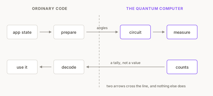
1. App state. Your application has some state: a request, a dataset or something a user just did.
2. Prepare. Ordinary code turns that state into numbers the circuit can take, usually angles.
3. Circuit. The circuit runs on the backend: a quantum computer, or a simulator of one.
4. Measure. Each shot ends in a measurement that reads one bitstring, and the tally of those bitstrings, the counts, comes back to your program.
5. Decode. Ordinary code turns the tally into a value the rest of your program can use.

Steps three and four run on the backend, and you reach them through one function call.

In the Oracle, the application state is the day's market data. The prepare step turns that data into the coefficients of a portfolio-optimization problem, and the coefficients set the circuit's rotation angles. IonQ runs the circuit and sends back a tally of sampled portfolios. In each 14-bit string, eight bits mark which of the eight candidate assets that portfolio holds.

The decode step measures the quality of the sampled portfolios and blends it with eight market signals into the risk score. The pipeline is built to publish the risk score to an Ethereum test network, where other programs can read it.

In the Oracle's listing, the function call between the two sides is backend.run, with the circuit built above it and the tally read below it:

qc = build_circuit(gammas, betas, ising_h, ising_J_pairs, SNAPSHOT)
job = backend.run(transpile(qc, backend), shots=SHOTS)
while job.status() is not JobStatus.DONE:
    time.sleep(2)
counts = job.result().get_counts()   # sampled portfolios -> risk score (BPS)

A music studio, a market tool and an artwork

Musiq, Quantum Regime Radar and Quantum Butterfly Field were also built in spring 2026, in a few weeks each. All three have a listing on Qollab that you can run and fork.

• Musiq is a music studio in the browser that plays a circuit's outcomes as notes.
• Quantum Regime Radar is a market tool that scores a window of market returns against five volatility regimes taken from market history.
• Quantum Butterfly Field is an artwork in which five butterflies are five qubits, one of them damaged and then recovered.

Figure 3 lines the three programs up against the five steps.

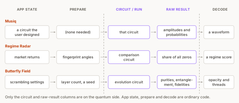
All three programs use more than a tally. Musiq and Butterfly Field read values that only a simulator can hand back, such as amplitudes, phases and purities. The Radar computes exact overlaps to rank its regimes before it spends any shots. Lesson 2 covers when a program can have those values.

Musiq

Tomoya Hatanaka, who led Musiq, wanted music generated directly from quantum states, because he finds music built on classical random-number generators repetitive. Emmanuella Adams, a creative technologist, worked on how circuits become sound and on the studio's interface.

Curiosity, not fear. Quantum computing is often presented as this impossible, gatekept thing. I want someone to hear their circuit and think, "Oh, that's mine. I made that." The feeling of creating something you don't fully understand yet. That is where learning starts.

Musiq has no separate prepare step, because the circuit you design in the studio is its input. Musiq's decode step is a mapping table. Each measured outcome picks which note plays, how often the outcome came up sets how strong that note is, and the statevector's phases shape how the notes interfere. The output is a waveform you can play and export.

Quantum Regime Radar

The Radar's premise is that a volatility model fitted in a calm market breaks in a crisis, so a modeller needs to know which regime the market is in first. Two of its five regimes are the low-volatility rally of 2017 and the 2020 COVID crash. The regime library is built on Alireza Khodaei's doctoral research, which estimated volatility-model parameters on a quantum annealer. An annealer is a different kind of quantum machine from the gate circuits in this course.

We have a bunch of known market regimes with respect to volatility, and we make a quantum fingerprint out of each. Then, given live data: how similar are these two days to the pre-crisis regime? There is no yes-or-no answer. There is a probability.

The Radar's prepare step turns a window of market returns into the angles of a circuit whose state encodes how the market's volatility has behaved, a fingerprint of those conditions. The playground cell ships those angles already fitted.

The circuit prepares that fingerprint, runs a reference regime's circuit backwards over it, and measures. Running a circuit and then its reverse returns every qubit to 0, the way two h gates in a row do. So when the two fingerprints are identical, every shot on a noise-free simulator reads all zeros. The decode step reads the share of all-zero shots as a similarity score.

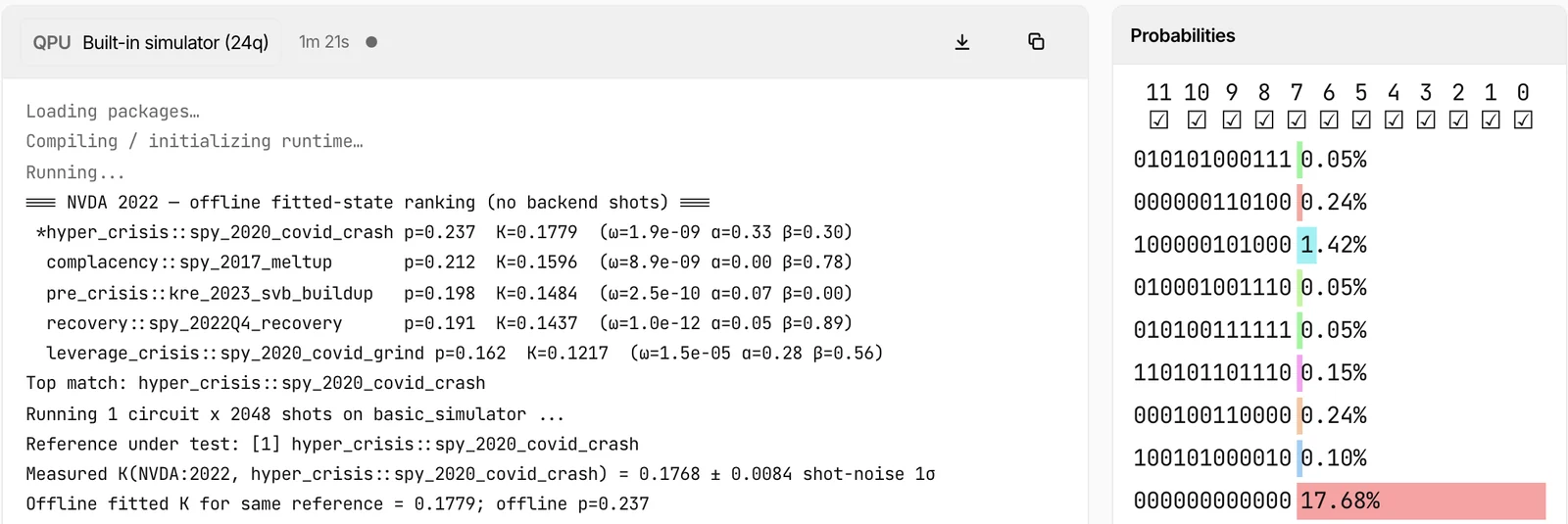
Figure 5 shows our run of the Radar on 22 September 2026, for NVDA in 2022, on the built-in simulator. The console shows the exact ranking first, with the COVID crash on top, then tests the top-ranked regime with one circuit. In the Probabilities panel, 17.68% of the 2,048 shots came back all zeros. The console reports that share as K = 0.1768, within shot noise of the exact 0.1779.

Quantum Butterfly Field

Xinyi Zhang, an artist and technologist, first painted Butterfly Field in 2024, while she lived on Oʻahu. She had the idea for the circuit after reading a Scientific American article on the quantum no-butterfly effect, a 2020 result by Yan and Sinitsyn. Once information is scrambled deeply enough across an entangled system, damage to one part cannot destroy it, and running the scramble backwards recovers the damaged part almost completely.

The one rule I held onto throughout was that every visual parameter had to be driven by a real quantum value, nothing decorative, nothing faked. The wing opacity really is the purity, the threads really are the mutual information between the qubit pairs. When something didn't look right, the solution was not to invent a prettier number, but to find a better mapping. The beauty had to be grounded in the physics.

Butterfly Field's prepare step picks a scrambling depth and a random seed, which fix the circuit's gates. The circuit scrambles the five butterflies into one field, damages one of them, and runs the scramble backwards. For each layer, the simulation returns every butterfly's purity, how much each pair of butterflies shares, and a fidelity for how far the damaged butterfly has recovered. The final fidelity comes from recorded runs on IonQ Forte hardware. The decode step turns those numbers into the picture, and the fidelity, for instance, sets how brightly the damaged butterfly glows.

Find the boundary in Quantum Garden

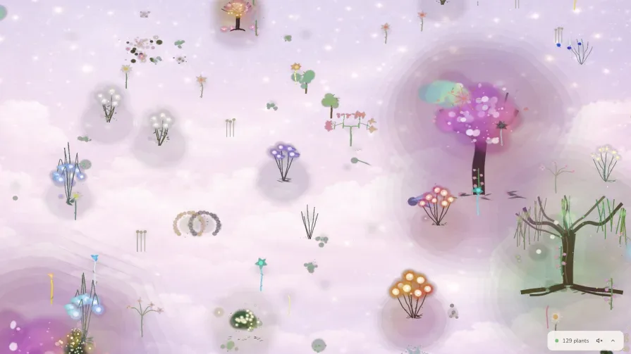
Amber Wang and Justin Pincar, a data scientist and a software engineer, built Quantum Garden, a digital garden where every plant gets its form from a circuit. They wanted to see what a garden based on the randomness of quantum measurement would look like. Neither came from quantum research. Justin had followed quantum computing for years before access to real hardware and the garden idea got him building.

Designing for quantum means treating concepts like superposition, entanglement, and probabilistic measurement as actual creative materials, not just technical details. Instead of thinking, "What output do I want?" you're asking, "What distribution of possible states do I want, and how should people encounter those states over time?"

Quantum Garden's listing on Qollab is about eighty lines and uses four gates, all of which you met in Course 2. The excerpt below shows the first three of the listing's six layers, verbatim. The other three add phases, a second entangling pass and a final rotation, all from the same seed.

seed = 42  # Each plant gets a deterministic seed from its ID hash

circuit = QuantumCircuit(5, 5)

# Layer 1: Full superposition — all 32 outcomes initially possible
for i in range(5):
    circuit.h(i)

# Layer 2: Seed-based Ry rotations — parameterized bias per qubit
for i in range(5):
    angle = (seed * (i + 1) * 0.1) % (2 * math.pi)
    circuit.ry(angle, i)

# Layer 3: Linear entanglement chain — correlates neighboring qubits
for i in range(4):
    circuit.cx(i, i + 1)

The prepare step is that seed. The listing's comment says each plant's seed comes from its ID hash, and the seed sets every rotation angle in the circuit.

The listing's own header says the circuit's layers create a "quantum fingerprint" that determines a plant's glyph pattern, colour palette, growth rate and opacity. The decode step that turns the fingerprint into those traits lives in the garden's app, outside the eighty lines you are looking at. Five qubits give thirty-two possible outcomes, and each plant's traits come from one of them. The app draws that outcome from a pool of results computed in advance, which lesson 4 comes back to.

Open the project, press Run on Qollab, and pick IonQ Aria 1 (25q) under Remotely Run Simulators in the Run Experiment dialog, then press Run.

The IonQ Aria 1 (25q) row under Remotely Run Simulators is IonQ's simulator with a noise model of the Aria 1 machine, and it is free. The same name appears again further down under Quantum Computer, which is the real machine and costs credits. Every run we pressed for this course used a simulator.

The first press takes a while, because the browser loads Python and Qiskit before anything runs. Ours took over a minute.

In our run on 22 September 2026 the console ended like this:

Job status is JobStatus.DONE
Counts for 100 shots: {'00001': 13, '00011': 15, '01001': 7, '01101': 24, '11101': 10}

Only the Counts line carries a result back from IonQ. The counts on that line add up to 69 of the 100 shots.

Takeaway

In the Qollab listing of each of the five projects, a backend.run call hands the circuit to a backend, and the result comes back across that call as ordinary data. To read a quantum application you did not write, find that call first, then read what the program feeds into it and what it makes of the result.

Lesson 2 presses Quantum Garden again and shows where the 31 shots missing from its tally went.