Quantum Optimization and QAOA

Quantum optimization means using a quantum computer to find the best of a huge number of possible answers, such as the best way to split a graph into two groups. QAOA, the standard circuit for quantum optimization, changes how often each answer comes out when you measure, and two adjustable angles set by how much.

The smallest version has one qubit, three gates and a measurement, and its two angles take that qubit from a 50/50 outcome to a certain one. Every circuit on this page is that same circuit on more qubits, sometimes stacked in more than one layer, up to a graph of twenty-four nodes.

What is quantum optimization?

MaxCut, the running example, is the problem of splitting a graph so that as many edges as possible run between the two groups. Every other problem on this page is rewritten into the same form.

One layer of the MaxCut circuit needs one two-qubit interaction per edge and one rotation per node. Only two numbers in that layer are free to change, the angles.

Annealing, the slow-cooling idea

Annealing is the metalworker's way of making steel that bends without breaking: heat it, then cool it slowly. A blade plunged into water from red heat comes out hard and brittle, because the atoms freeze in place, defects and all.

Cooled slowly, the same steel settles into a lower-energy arrangement, because at each temperature the atoms still have enough motion to leave a bad position for a better one.

In 1983 Kirkpatrick, Gelatt and Vecchi turned annealing into an algorithm. Simulated annealing starts from a random answer and accepts a worse neighbouring answer with a probability that shrinks as a temperature variable drops. Simulated annealing ends up in a good answer for the same reason the slowly cooled steel does.

Adiabatic quantum computation, proposed in 2000, is the quantum version of cooling slowly. A Hamiltonian is a problem's cost written as an energy, and its ground state, the lowest-energy state, encodes the best assignment.

Start in the easy ground state of one Hamiltonian and change that Hamiltonian into the problem's; if the change is slow enough, the state stays close to the ground state throughout.

QAOA cuts the adiabatic path into a fixed number of layers and lets a classical optimizer choose the two angles of each layer. Farhi, Goldstone and Gutmann showed that with enough layers the circuit can follow the adiabatic path.

A single layer is the fast-cooling version. On a 24-node graph from a published project, one tuned layer raises the average cut from the 18.5 edges of a random split to 25.5, out of a possible 33.

Where quantum optimization came from

Six dates, from simulated annealing to the current scaling experiments:

The 2014 paper proved a guarantee: on any graph where every node has three edges, one QAOA layer at its best angles gives samples that average at least 0.6924 times the best possible cut.

A month later the same three authors showed one layer beating the best known classical guarantee on a constraint problem called E3LIN2. By May 2015 a classical algorithm had a better guarantee, so the lead lasted five months. The QAOA bound remains proven; it is no longer the best known.

What one layer does

One QAOA layer works on the two numbers a qubit has for each outcome it can give. The weight says how often that outcome comes back when you measure. The phase is an angle that measurement never shows, and the cost step works on that one. Two qubits have both numbers for four outcomes, three qubits for eight, and twenty-four qubits for sixteen million.

One QAOA layer is two steps. The cost step changes only the phases; the mixer step changes the weights.

In the cost step, every outcome's phase turns by an amount set by that outcome's score. A good outcome and a bad one end up with different phases, and nothing else has happened: measure now and the counts are exactly what they were before.

In the mixer step, phase differences become weight differences. Outcomes whose phases were turned one way gain weight and outcomes turned the other way lose it. The two angles decide how far the phases turn and how much weight follows: gamma for the cost step, beta for the mixer step.

On one qubit, with a score that prefers 1, four panels show each step, and what smaller angles do:

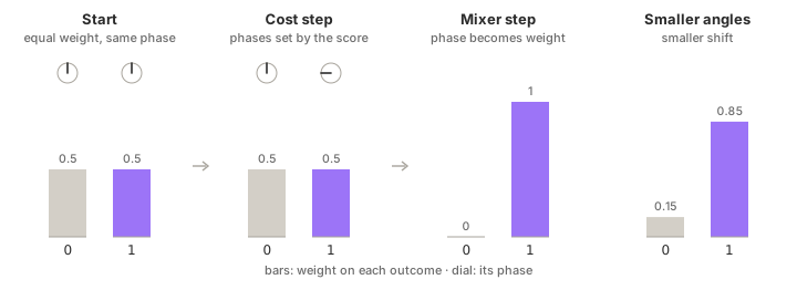
Both bars start at one half with the same phase. After the cost step the dial over 1 has turned and both bars are unchanged. After the mixer step the weight has moved, and at the right pair of angles all of it moves to 1; at smaller angles, less of it. Measure a thousand times and the counts follow the bars.

Three gates reproduce the first three panels on one qubit, and a measurement reads the bars.

The smallest circuit you can make

A cost that prefers 1 is one rz, the mixer is one rx, and measuring reads the bars. The run button under this listing and the next opens Qollab's showcase-qaoa-qubo example: fork it, paste the listing over the example's code, and run the listing.

​# 'backend' is pre-created for you in the Qollab Playground.
​from math import pi
​from qiskit import QuantumCircuit
​​
1gamma, beta = -pi / 4, pi / 4
​​
​qc = QuantumCircuit(1, 1)
2qc.h(0)
3qc.rz(2 * gamma, 0)
4qc.rx(2 * beta, 0)
​qc.measure(0, 0)
​​
5print(backend.run(qc, shots=1000).result().get_counts())
1The two angles. This pair is exact for one qubit: every shot will read 1.
2Equal weight on 0 and 1, the starting point of every QAOA circuit on this page.
3The cost step writes the score into the phase: the 1 half of the state gets a different phase from the 0 half. Nothing in the counts has changed yet. Qiskit's rotation gates take twice the angle, a convention every listing here follows.
4The mixer step turns that phase difference into a weight difference.
5{'1': 1000}: every shot reads 1. Set gamma to +π/4 and every shot reads 0; halve either angle and 1 comes back about 85% of the time.

One qubit has nothing to cut, so the score there is a preference. The first problem with something to cut is one edge between two nodes: it is cut when the two bits differ, so 01 and 10 are the answers and 00 and 11 are not. The circuit adds one two-qubit interaction for the edge, written as a three-gate sandwich, and keeps its two angles:

​# 'backend' is pre-created for you in the Qollab Playground.
​from math import pi
​from qiskit import QuantumCircuit
​​
1gamma, beta = -pi / 4, pi / 8
​​
​qc = QuantumCircuit(2, 2)
2qc.h([0, 1])
3qc.cx(0, 1)
​qc.rz(2 * gamma, 1)
​qc.cx(0, 1)
4qc.rx(2 * beta, [0, 1])
​qc.measure([0, 1], [0, 1])
​​
5print(backend.run(qc, shots=1000).result().get_counts())
1The two angles. This pair is exact for one edge: every shot will cut the edge. The mixer angle is π/8 here, not the π/4 of the one-qubit circuit: with two qubits the exact pair moves, and the heatmap after this listing maps every pair. Change either angle and the counts change.
2Even weight on all four strings: 00, 01, 10, 11. The standard QAOA circuit starts here.
3The cost step for one edge. The cx, rz, cx sandwich shifts the phase of a string by an amount that depends on whether its two bits differ. Cut strings get one phase, uncut strings the other.
4The mixer step. A rotation on each qubit that turns the phase difference the cost step set into a weight difference. Phases alone change no count; this step turns them into counts.
5{'01': 503, '10': 497}: about half each, and no 00 or 11 at all. No shot returns an uncut edge.

Flip the sign of gamma and the counts flip with it: all 00 and 11, an uncut edge on every shot. Set both angles to zero and the four strings come back at a quarter each. Halve gamma to −π/8 and the cut strings get 85% of the weight instead of all of it.

All four results come from the same gates; only the two numbers changed. The angles set what a QAOA circuit computes, and for one edge the average cut at every pair of angles fits in one figure:

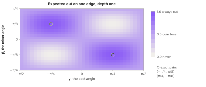
The row and the column through the centre are both at one half. At beta = 0 the mixer does nothing and the cost step's phases never reach the counts. At gamma = 0 there are no phases to turn into weight.

The counts move away from a quarter each only when both angles are away from zero, and the peak or trough the pair sits in decides whether the cut strings or the uncut strings come out.

The official showcase-qaoa-qubo example is this same problem, written as maximize x + y - 2xy and handed to Qiskit's QAOA class, with COBYLA, a classical optimizer from SciPy that needs no gradients, tuning the angles over at most fifty evaluations. Run the example and 01 and 10 get almost all the weight: COBYLA has found one of the two peaks.

Turning a problem into a cost

Between one edge and a full graph comes the bookkeeping: the problem has to become a number that a string of bits can be scored by, and the score has to become the phases in the cost step. The standard form, used by every project on this page, is a QUBO, quadratic unconstrained binary optimization: pick 0 or 1 for each variable to minimize a polynomial with single terms, pairwise terms and nothing higher.

Flip the sign and a score to maximize becomes a cost to minimize, so MaxCut fits the form. Qollab's showcase-qubo-exact, one of the official Playground examples, builds a QUBO with three variables and prints the score of every one of its eight strings. The listing starts after the file's imports, so run the example itself rather than pasting this one:

​# minimize -x - 2y - 3z + 2xy + 2yz
​# (each variable wants to be 1, but x-y and y-z "repel" each other)
​qp = QuadraticProgram("qubo")
​qp.binary_var("x")
​qp.binary_var("y")
​qp.binary_var("z")
1qp.minimize(linear={"x": -1, "y": -2, "z": -3}, quadratic={("x", "y"): 2, ("y", "z"): 2})
​print(qp.prettyprint())
​​
​# Brute-force all 8 assignments - only possible because the problem is tiny
​print("\n x y z   objective")
2for bits in product((0, 1), repeat=3):
​    value = qp.objective.evaluate(list(bits))
​    print(f" {bits[0]} {bits[1]} {bits[2]}   {value:+.0f}")
1Each single term rewards a variable for being 1. Each pair term is a penalty for two of them being 1 together. A graph's edges are exactly a set of pair terms.
2Eight strings for three bits. The loop scores every one, and no solver can do that once the string is long: at sixty variables the table has more rows than there have been seconds since the Big Bang.

The table the example prints has eight rows, and one of them, 1 0 1, reaches −4:

 x y z   objective
 0 0 0   +0
 0 0 1   -3
 0 1 0   -2
 0 1 1   -3
 1 0 0   -1
 1 0 1   -4
 1 1 0   -1
 1 1 1   -2

No other row reaches −4. That number is the ground truth for this example, and every quantum run on this page has a ground truth of its own. The file's own header comment calls the exact answer "the trusted baseline every quantum solver gets measured against".

To become phases, the 0/1 variables become spins, variables that are +1 or −1. The substitution is x = (1 - z) / 2: a bit that is 0 becomes a spin that is +1 and a bit that is 1 becomes −1. A pair term x·y becomes (1 − z_x − z_y + z_x·z_y) / 4: a constant, a term on each spin, and a z·z term.

The z·z term is the product of the two ±1 signs that two measured bits map to. The cx, rz, cx sandwich in the one-edge circuit gives that product a phase. So an edge of the graph becomes one two-qubit interaction in the circuit, and a variable's own reward becomes a single-qubit rotation, the rz from the one-qubit circuit.

The gates in these circuits

Four gates and one instruction cover every excerpt on this page.

Two angles, sixteen million splits

Dr. Siti Fariya's Quantum Courier is a browser game that races classical and quantum solvers across five logistics problems, and its fourth stage is MaxCut on twenty-four nodes. The Playground version is the script the project publishes for that stage's run on IonQ Forte, a trapped-ion quantum computer.

The script's circuit is the one-edge circuit with the cost sandwich repeated for every edge and the mixer repeated for every node:

​def qaoa_circuit(gamma, beta):
​    qc = QuantumCircuit(N_NODES, N_NODES)
​​
​    # Initial state: equal superposition
1    qc.h(range(N_NODES))
​​
​    # Cost layer: e^{-i gamma C}
2    for (u, v) in EDGES:
​        qc.cx(u, v)
​        qc.rz(2 * gamma, v)
​        qc.cx(u, v)
​​
​    # Mixer layer: e^{-i beta B}
3    for q in range(N_NODES):
​        qc.rx(2 * beta, q)
​​
​    qc.measure(range(N_NODES), range(N_NODES))
​    return qc
1Twenty-four Hadamards, and the register holds equal weight on all 16,777,216 splits.
2One sandwich per edge, thirty-seven of them. Each shifts a split's phase by an amount that depends on whether that edge is cut, so a split's total phase depends only on how many edges it cuts.
3One rx per node, the same mixer as before. Still the only place weight moves between splits.

The graph is the twenty-four-node one from the opening: thirty-seven edges, a ring with chords across it. Scoring all 16,777,216 splits takes a laptop under a second. A random split cuts 18.5 edges on average, no split cuts more than 33, and exactly six splits reach that.

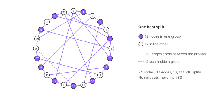
Scoring is classical code. For each measured string the script counts the edges whose two ends are on different sides, then averages over the shots:

​def cut_value(bitstring):
​    # Qiskit returns bitstrings in reverse: bit i lives at position N-1-i
1    bits = [int(b) for b in bitstring[::-1]]
2    return sum(1 for (u, v) in EDGES if bits[u] != bits[v])
​​
​​
​def expected_cut(counts, shots):
3    return sum(cut_value(bs) * c for bs, c in counts.items()) / shots
1A measured string is one split of the graph. Reversing the string is a Qiskit convention: qubit 0 is the last character.
2The cut: one point per edge whose ends disagree. This is the score, and no qubit is involved in it.
3The average over every shot, the number an optimizer works from.

On an exact simulator, which keeps the weight of every split rather than sampling, the circuit's output distribution can be computed for any pair of angles, and every split can be scored, so the figure compares two pairs.

Grey is a random split, or equally the circuit with both angles at zero. Purple is the pair an exact-simulator search over both angles finds best for this graph, rounded to two decimals: gamma = -0.30, beta = 0.39.

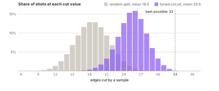
One layer moves weight off the bad splits and onto the good ones, and the average moves seven edges to the right. The circuit returns no single answer; the best split becomes a more frequent sample.

A sample from the tuned circuit is optimal about once in a thousand shots, against once in 2.8 million for a random split. In a 4,096-shot job the best split therefore shows up about four times, and the best string in the tally is the best split on almost every run.

The table is one layer on the same 24-node, 37-edge instance at four pairs of angles, every row derived from the exact distribution. In the table, gamma is the cost angle and beta the mixer angle, and the last column is the best cut you can expect to see in a job of 4,096 shots. The best possible cut is 33:

On twenty-four nodes the pair that is exact on one edge leaves the average at 18.5, the same as a random split, and makes the best split rarer. Which angles are best depends on how many edges meet at each node, so angles do not transfer from a toy to a real instance.

And the sign pairing matters as much as the size. With gamma flipped the same circuit averages 11.5 edges, well below a random split, because the circuit is now concentrating weight on the splits that cut the fewest edges.

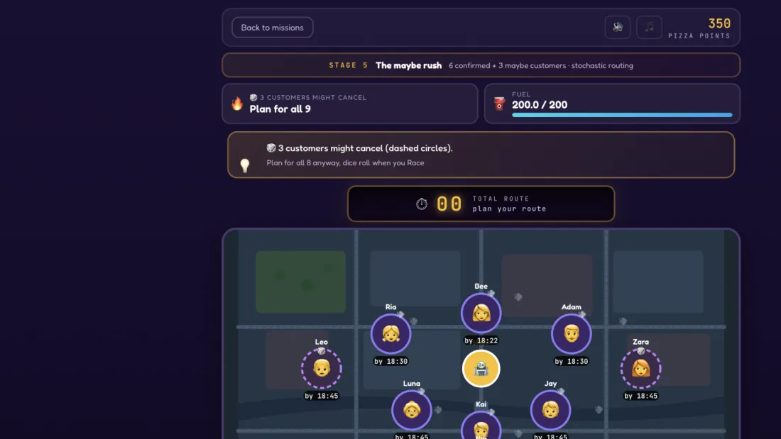Quantum CourierDr. Siti Fariya · u/Sitifar · Python + QiskitDr. Siti Fariya built a browser game that races classical and quantum solvers across five real logistics problems, and shows honestly which one wins, and why.

The loop runs on the simulator

Finding the purple pair is the classical optimizer's job. The loop itself is ordinary code, and each step of it runs the circuit once. Starting from a guess, the optimizer runs the circuit at that pair and reads the average cut. Then the optimizer adjusts the pair and runs again: fifty times in the repository version of Quantum Courier's optimizer and in the official example, a few hundred per start in the Oracle, which restarts from several seeds.

When the budget runs out the optimizer returns the best pair it found. Quantum Courier's script defines the objective that loop calls.

For a single Forte job the script skips the loop and fixes GAMMA_STAR and BETA_STAR before submitting, with a comment that says so. In a fork, the pairs from the table go into those two constants.

The objective itself wraps one run:

​def objective(params):
​    """Negative expected cut — minimised by COBYLA."""
1    bound = template.assign_parameters({gamma_p: params[0], beta_p: params[1]})
2    job = backend.run(bound, shots=SHOTS)
​    counts = job.result().get_counts()
3    return -expected_cut(counts, SHOTS)
1One candidate pair of angles goes into the circuit template.
2One evaluation is one job of 4,096 shots. On hardware each evaluation is a queued, paid job, and an optimizer typically needs fifty of them.
3The average cut, negated because COBYLA minimizes. The optimizer works from this number alone.

Fifty evaluations at 4,096 shots is 204,800 shots for two numbers, and on a shared machine each evaluation waits in a queue. So both hardware projects on this page tune their angles on a simulator and send the finished circuit to the machine once.

Jamie Dominguez's Quantum Systemic Oracle picks a portfolio of eight crypto assets the same way, with a QUBO built from market data.

The circuit the Oracle sends to the machine has fourteen qubits: one decision qubit per asset, plus six that hold market state. The tuning runs on the eight asset qubits alone, inside the Playground file, with Nelder-Mead, a classical optimizer written out in plain Python in the file.

The optimizer scores each candidate pair like this. h holds one number per asset and J_pairs one number per pair of assets, the two kinds of term the cost is made of:

​def optimize_angles(h, J_pairs, n, layers) -> Tuple[List[float], List[float], float]:
​    """Best (gammas, betas) by multi-start Nelder-Mead on <H_C>."""
​    H = build_hamiltonian(h, J_pairs, n)
​​
​    def energy(angles: List[float]) -> float:
​        gammas, betas = angles[:layers], angles[layers:]
​        sv = Statevector.from_instruction(
1            asset_only_qaoa_circuit(gammas, betas, h, J_pairs, n))
2        return float(np.real(sv.expectation_value(H)))
1The full state of the eight asset qubits, computed exactly. No shots and no noise, so each step is cheap enough to take hundreds of them.
2The average cost under that state, read straight off the weight of every string. A real machine can only estimate this number from a tally.

Three ways of running a circuit appear in these projects. An exact simulator keeps every weight and needs no shots; the Oracle's tuner uses one. A sampled simulator returns a tally the way hardware does, with shot noise but none of the device's.

The machine itself returns a tally with the device's noise in it. Courier's script sets its own provider and backend to IonQ Forte; with those two lines removed in a fork, its objective, which always asks for shots, runs on whichever backend the Playground provides.

On an exact simulator the objective is exact. On hardware, or on any simulator that samples, the objective is an estimate, and how good an estimate is a number you can derive. At the tuned pair a single sample's cut has a standard deviation of 2.6 edges. Over 4,096 shots the average is known to about 0.04 of an edge, one standard error.

Shot noise is a small part of the cost of the loop. Most of the cost is that every evaluation is a job, and that the landscape of angles has the shape of the one-edge heatmap with more peaks and troughs.

Constraints become penalties

The Oracle's problem is portfolio selection: which of eight crypto assets to hold, given their expected returns and how their prices move together. A budget rule says how many to hold, and a QUBO has no constraints by definition, so the rule has to become part of the cost. The file folds the rule in like this:

​Q = [[0.0] * n for _ in range(n)]
​for i in range(n):
1    Q[i][i] += lam * var[i] - mu[i] - ALPHA_POLY * poly[i] + BETA_FUNDING * fnd[i]
​    Q[i][i] += ALPHA_DISAGREE * disagree[i] - ALPHA_SIDEWAYS * sideways[i] + macro_tilt
​    for j in range(n):
​        if i != j:
2            Q[i][j] += lam * corr[i][j] * math.sqrt(var[i] * var[j])
​for i in range(n):
3    Q[i][i] += BUDGET_PENALTY * (1 - 2 * k_target)
​    for j in range(n):
​        if i != j:
​            Q[i][j] += BUDGET_PENALTY
1The single terms: one number per asset from its own return, risk and market signals.
2The pair terms. Two assets that move together are penalised for being held together, the diversification rule from Markowitz's portfolio theory written as a QUBO.
3The budget rule, folded into the cost rather than checked outside it: a term per asset that depends on the target count k_target, and a term per pair that adds a cost for holding two assets at once. The count of assets held enters the cost as a price; nothing enforces it.

Converting to spins uses the same substitution, x = (1 - z) / 2, named in the file's own comment, and the file then rescales the result, a step the one-edge circuit did not need:

​# QUBO -> Ising via x_i = (1 - Z_i) / 2
​h = [0.0] * n
​J = [[0.0] * n for _ in range(n)]
​for i in range(n):
1    h[i] += -Q[i][i] / 2.0
​    for j in range(n):
​        if i != j:
​            h[i] += -Q[i][j] / 4.0
2            J[i][j] += Q[i][j] / 4.0
​J_pairs = [{"i": i, "j": j, "value": J[i][j] + J[j][i]}
​           for i in range(n) for j in range(i + 1, n)]
​​
​# Normalize so the largest |coeff| ~ 1 (keeps QAOA angles meaningful; the
​# classical optimum and reported costs always use the raw Q matrix).
​scale = max([abs(x) for x in h] + [abs(p["value"]) for p in J_pairs] + [1e-9])
​return {
​    "lambda": lam,
​    "target_k": k_target,
​    "Q_matrix": Q,
3    "ising_h": [x / scale for x in h],
​    "ising_J_pairs": [{"i": p["i"], "j": p["j"], "value": p["value"] / scale} for p in J_pairs],
​}
1Each variable's own reward becomes a field on one spin: a single-qubit rz in the cost step.
2Each pair term becomes a coupling between two spins: one cx, rz, cx sandwich.
3Every field and coupling divided by the largest of them, so the biggest coefficient is about 1. gamma multiplies every coefficient, so without this the useful range of gamma would depend on the units the returns were quoted in.

With the fields and couplings computed, the layer itself is the Courier loop with one extra line, in its general form:

​def apply_cost_layer(qc, gamma, h, J_pairs, n):
​    for i in range(n):
1        qc.rz(2.0 * gamma * h[i], i)
​    for pair in J_pairs:
​        i, j, v = pair["i"], pair["j"], pair["value"]
​        qc.cx(i, j)
2        qc.rz(2.0 * gamma * v, j)
​        qc.cx(i, j)
​​
​​
​def apply_mixer_layer(qc, beta, n):
​    for i in range(n):
3        qc.rx(2.0 * beta, i)
1The field on each spin, scaled by gamma. MaxCut had none of these; a portfolio has one per asset.
2The coupling, scaled by gamma and by its own strength. On the MaxCut graph every coupling was the same size; here each pair has its own.
3The mixer does not change with the problem. Only the cost step depends on what is being optimized.

Every pair of the eight assets gets a coupling, twenty-eight in all, so one cost step is 56 cx gates, the figure the project's README gives for one layer.

The six extra qubits the project measures alongside the eight asset qubits hold market state and are prepared with single-qubit gates only. The project's showcase describes that single-qubit preparation as the choice that keeps the circuit growing by one qubit per asset rather than per signal.

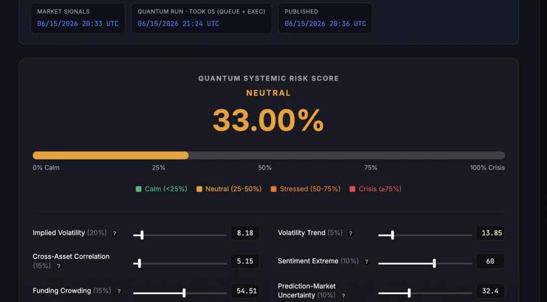Quantum Systemic OracleJamie Dominguez · u/jamie · Python + QiskitBlockchain oracle that publishes a quantum-computed 'systemic risk score' for crypto markets every day. Smart contracts and prediction markets can use the quantum-derived risk data as a primitive. Commoditizing quantum compute as an on-chain data feed.

What approximate means

Two numbers set the expectations for one layer of QAOA. Farhi, Goldstone and Gutmann's guarantee is an average cut, at the best angles, of at least 0.6924 times the best possible on any graph where every node has three edges. Goemans and Williamson's classical algorithm from 1995 guarantees 0.878.

On the Courier graph the tuned layer averages 25.5 of a possible 33, which is 0.77. Greedy local search from a random split, flipping any node whose flip cuts more edges until nothing improves, averages about 31 on the same graph and reaches 33 within a few restarts, in milliseconds.

So on this graph the average sample from one layer is worse than what a classical heuristic returns. On any problem small enough to score exhaustively, that comparison can be made exactly.

Quantum Courier's README says which stages the classical solvers win, and reports the vehicle-routing stage where four QAOA variants lost on Forte to classical simulated annealing, a result the project left in the game on purpose.

A QAOA run therefore reports the best string in the tally, checked classically, rather than the average. The Oracle's file shows that step; ranked is its tally with the strings below a noise floor already removed:

​nonempty = [(b, c) for b, c in ranked if any(b)]
​rec_pool = nonempty or ranked
1rec_bits, rec_count = min(rec_pool, key=lambda kv: classical_cost(list(kv[0]), Q_matrix))
​top_bits = list(rec_bits)
​top_held = [ASSETS[i] for i, b in enumerate(top_bits) if b]
​top_cost = classical_cost(top_bits, Q_matrix)
2gap = (top_cost - opt_cost) / abs(opt_cost) * 100.0 if opt_cost else 0.0
1Every sampled portfolio above the noise floor is re-scored with the classical cost function, and the cheapest non-empty one, if any, is the recommendation. The most frequent string is printed for reference; the recommendation is the cheapest one.
2The gap to the brute-force optimum over all 256 portfolios. At eight assets the true answer is checkable, so the quantum run is measured against it.

The gap to the optimum feeds what the README calls a solver-quality signal, weighted at 5% of the Oracle's published index so that, in the README's words, the headline number "never hinges on solver perfection, but degrades gracefully with it".

QAOA needs two things to beat the brute-force table: strings too long to score exhaustively, and enough layers to raise the average. Both depend on hardware.

Depth that helps on the simulator and hurts on the machine

Each extra layer adds another cost step and another mixer step with their own pair of angles. On an ideal simulator the best achievable average never falls as layers are added, and usually rises. How many layers there are is called p.

In the Oracle's file p is one constant, QAOA_LAYERS = 2, which sets how many angle pairs the optimizer returns, and the circuit is a loop over those pairs:

​def asset_only_qaoa_circuit(gammas, betas, h, J_pairs, n):
​    qc = QuantumCircuit(n)
​    for i in range(n):
​        qc.h(i)
1    for layer in range(len(gammas)):
​        apply_cost_layer(qc, gammas[layer], h, J_pairs, n)
​        apply_mixer_layer(qc, betas[layer], n)
​    return qc
1One pass per layer, each with its own gamma and beta. Two layers means four angles to tune. The eight-asset cost step is 56 cx gates, so two layers are 112 and three are 168.

The project tested one, two and three layers on IonQ Forte and wrote down what happened. Its README reports that the binding constraint was two-qubit gate error, not circuit depth (the number of gate rounds the compiled circuit runs in sequence), and puts the usable limit at about ninety two-qubit gates.

One layer, at 56 gates, was the README's "fidelity-optimal hardware setting". Deeper circuits "look marginally better on the ideal simulator but flatten toward uniform on the QPU", the quantum processor.

Every two-qubit gate adds an error, the errors compound, and past a certain count the distribution the circuit was shaping is lost to the noise. On the Oracle's runs the distribution flattened back towards the uniform one the circuit started from.

Every QAOA run on today's hardware has to balance layers against gate errors. More layers can raise the ideal average and cost accuracy on the machine, and the layer count that is best on the simulator need not be the one that is best on the machine.

Google's 2021 experiment found the same pattern on a different machine. On its superconducting chip, problems whose graph matched the qubit wiring improved with more layers. Problems that needed extra gates to route around the wiring got worse as they grew.

IonQ Forte, a trapped-ion machine, connects every qubit to every other, so the Oracle's twenty-eight couplings need no routing and the limit is the gate count itself.

Tune and debug on the simulator, then use the machine for what it alone can answer: whether the distribution you shaped survives the gate count at the layer count you chose.

Start with one qubit

A quantum optimizer is a circuit whose shape is fixed by the problem and whose behaviour is fixed by a handful of angles. The problem becomes a cost, the cost becomes phases, and a mixer turns the phases into weight. A classical loop chooses the angles that push the weight towards the answers you want.

The run returns a tally, and the answer you keep is the best string in it, scored by ordinary code.

Start with the one-qubit circuit. Fork the QUBO-with-QAOA example, paste the one-qubit listing over its code, and run it; the counts can be predicted before the run. Set gamma to zero and 0 and 1 come back about equally; set it back to −π/4 and every shot reads 1, with every gate unchanged.

Then the one-edge listing the same way: at −π/4 and π/8 only 01 and 10 come back. Then Quantum Courier's script: in a fork, delete its own provider and backend lines so that the Playground's backend is used, put a pair from the table into GAMMA_STAR and BETA_STAR, run it on a local simulator, and the expected cut it prints matches the table's average to within a tenth of an edge.