Building with Quantum Entanglement

Entanglement is two or more qubits in one joint state that cannot be split into a separate state for each. For the pair built below, neither qubit has a definite value of its own until it is measured.

Measure both the same way and one result tells you the other, however far apart the qubits are. Nothing travels between them, and the effect cannot carry a message: to see the agreement, the two people measuring still have to compare results over an ordinary channel, no faster than light.

Entanglement is different from two matched gloves posted in two boxes, where each box held a definite glove all along and opening one only revealed it. An entangled pair holds no definite values before the measurement, and the answers still agree. The Bell state below shows how to tell the two apart.

Where entanglement came from

The argument started in 1935; John Bell showed in 1964 that it could be tested, and the first test ran in 1972.

Einstein called entanglement "spooky action at a distance" and held that the result was carried by some hidden detail the theory had missed.

Bell showed what Einstein's assumption implied: if the values were fixed in advance and nothing travelled between the particles, the correlations could not exceed a certain limit, and entangled pairs exceed it. In 2015, experiments at Delft, Vienna and NIST closed the last loopholes, the gaps that had left room for another explanation. Hidden details of Einstein's kind, local and fixed in advance, are ruled out.

The Bell state, the smallest entangled pair

Two qubits and two gates make an entangled pair: put one qubit into superposition with a Hadamard, then link it to the second with a CNOT.

​# 'backend' is pre-created for you in the Qollab Playground.
​from qiskit import QuantumCircuit
​​
​shots = 1000
1qc = QuantumCircuit(2, 2)
2qc.h(0)
3qc.cx(0, 1)
4qc.measure([0, 1], [0, 1])
​​
5job = backend.run(qc, shots=shots)
6counts = job.result().get_counts()
​print(counts)
1A circuit is a list of operations to run in order. This one asks for two qubits and two ordinary bits: the qubits do the quantum work, and the bits are storage for the answers you read out at the end.
2A gate is one operation applied to a qubit. This is the Hadamard, applied to qubit 0, and it leaves that qubit in superposition: no fixed value, equally likely to read 0 or 1 once you measure it.
3This line entangles the pair. CNOT is a two-qubit gate: the first argument is the control, the second is the target, and it flips the target on every branch where the control reads 1. Because qubit 0 has no fixed value yet, both branches survive, and the two qubits end up sharing one state.
4Measuring is the only way to see a qubit, and it forces each one to a definite 0 or 1. This copies qubit 0 into bit 0 and qubit 1 into bit 1.
5Send the circuit to a real quantum computer, or to a simulator. One run gives one pair of bits and which pair is random, so you run it 1,000 times to see the pattern. Each run is called a shot.
6Tally those 1,000 results. A dict like {'00': 502, '11': 498} means 502 runs gave both qubits 0 and 498 gave both 1; the order of the keys can vary.

|00⟩ means both qubits came out 0. About half the shots come back 00 and half 11, never 01 or 10. Which one you get is random, but the two always agree. On real hardware a few mismatched shots appear; they come from device noise, and an ideal Bell state produces none.

Those counts alone do not prove entanglement: two gloves give the same 00 and 11. A basis is the question you put to a qubit, and "are you 0 or 1" is only one of them.

The second-basis test asks a different one: fork the Bell state and add qc.h(0) and qc.h(1) before the measurement. The pair still agrees every time. Two gloves, each already 0 or 1, come out of the two Hadamards as independent coin flips, so their answers agree only half the time.

The gates in these circuits

Five gates cover every excerpt in the sections that follow, and three of them are the ones you ran above. The full projects use a few more, mostly other rotations.

Quantum Market Game, a two-qubit visualiser, Entangled Body, Quantum Garden, Quantum Patterns and Quantum Butterfly Field each use an entangling operation.

Quantum Market Game: correlated buy and sell decisions

Quantum Market Game puts two traders' buy-or-sell decisions on two qubits and lets you entangle the pair before the market opens. Selling while the other buys pays the most; if both sell, they both lose money. With the pair entangled, their choices can come out correlated instead of independent.

Each trader is a qubit: |0⟩ means sell, |1⟩ means buy. A rotation sets the odds, so a trader can be mostly buy, mostly sell, or anywhere between.

Unless a trader's angle is set to certainty, both traders sit in superposition until the market opens, and measuring the pair fixes each decision.

​qc = QuantumCircuit(2, 2)
1qc.ry(angle_1, 0)
​qc.ry(angle_2, 1)
2if entanglement:
3    qc.cx(0, 1)
​qc.measure([0, 1], [0, 1])
1The angle sets this trader's odds, and it comes before the qubit. At 0 they are certain to sell, at π certain to buy, at π/2 the even 50/50 the Hadamard makes. In between it is not linear: the chance of buying is sin²(angle/2).
2All of the game's correlation comes from one optional line. With the flag off the two qubits stay independent and the round is ordinary game theory played with random draws.
3The same CNOT as the Bell state. At the file's default angles, 1.5707, which is π/2 to within a ten-thousandth, the CNOT has almost nothing to do: two qubits in the same even split are one of the inputs a CNOT leaves unchanged.

The game shows one basis only, buy or sell, and a table of correlated outcomes can always be reproduced by classical shared randomness, so the game cannot serve as a Bell test.

In the play_game(...) call at the bottom of the file, set angle_1=np.pi/2 and angle_2=0, where the CNOT changes the state, then run once with entanglement=False and once with entanglement=True. The payoff table changes between the two runs, and with entanglement on, the pair is a Bell state you could test in a second basis.

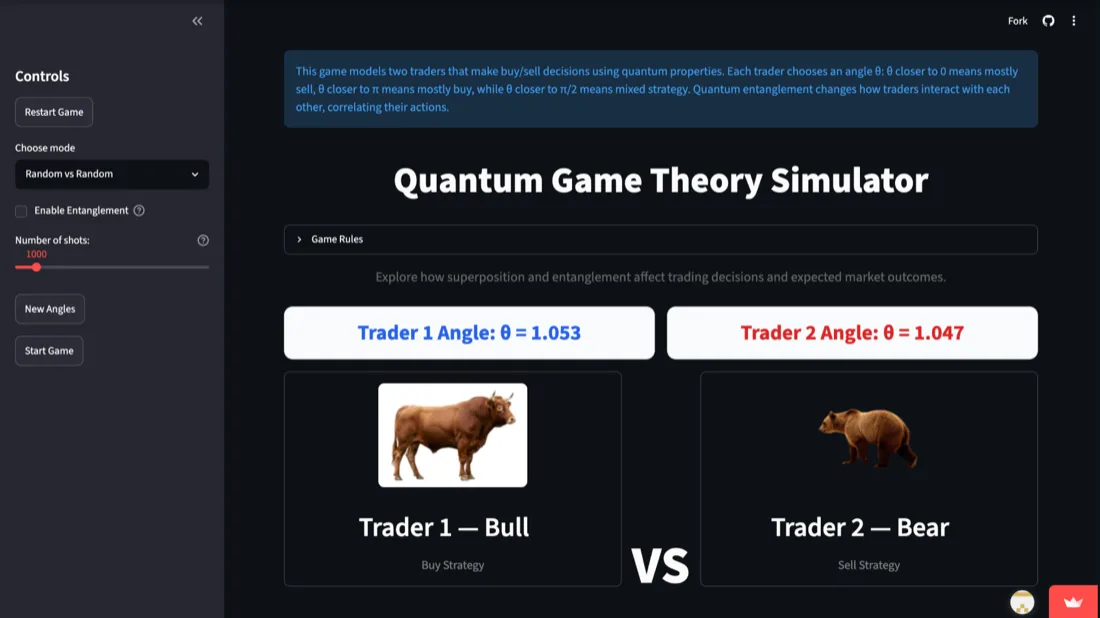Quantum Market GameAadarsh Venkat Ramanan · u/q-aad · Python + QiskitThe project is a twist on a classical game theory scenario: Prisoner's Dilemma.

A two-qubit visualiser: neither half has a state of its own

A Bloch sphere draws a single qubit's state as an arrow from the centre. Draw each qubit of a Bell pair on its own sphere and the arrow has zero length: neither qubit points in any direction by itself.

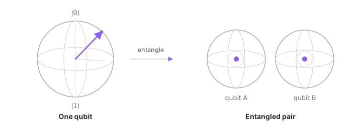
A two-qubit state like the Bell pair's is a list of four numbers. For a maximally entangled pair like this one, those numbers describe only the relationship between the qubits: the pair's state can be known completely while measuring either qubit alone gives an even split in every basis.

Onri Benally's visualiser draws the same pictures for two states so you can put them side by side: the plain |00⟩ state, where each qubit has its own direction, and a Bell pair.

The visualiser builds its Bell pair from the same two gates as the Bell state above, then adds a couple of single-qubit turns that leave the entanglement untouched.

Each state goes to a set of plotting functions. The excerpt is the opening of one of them, plot_steering_ellipsoid, which computes three parts of the state.

1    rho = state.data
​    # Calculate Bloch vectors and correlation tensor
2    a = np.array([np.trace(rho @ np.kron(s, np.eye(2))).real for s in pauli_matrices])
3    b = np.array([np.trace(rho @ np.kron(np.eye(2), s)).real for s in pauli_matrices])
4    T = np.array([[np.trace(rho @ np.kron(si, sj)).real for sj in pauli_matrices] for si in pauli_matrices])
1The density matrix: a 4 by 4 grid of numbers, the complete description of the two qubits together. state is whichever of the two states the visualiser was handed.
2a describes qubit A on its own. np.kron pastes two small matrices into one that acts on A and leaves B alone, and the trace against rho turns that into a single number. There is one number per axis, three in all, and for a Bell pair all three are 0.
3The same three numbers for qubit B, also all zero for a Bell pair.
4T describes both qubits at once: nine numbers, one for each pair of axes. On their own they prove nothing, since a plain |00⟩ has a 1 in there too. For the Bell pair they survive while a and b go to zero, so T can no longer be a times b.

Fork the visualiser and add print(title, a, b, T) after those lines, inside plot_steering_ellipsoid. The file calls that function once for |00⟩ and once for its final entangled state, so the console shows both.

For |00⟩, T is exactly a times b: the correlations two qubits that each point somewhere would give you anyway. For the entangled state a and b are zero and T is not, so no pair of individual directions can account for it.

Entangled Body: entanglement the counts do not show

Entangled Body is a 3D human figure whose regions are qubits, linked by entangling gates on the anatomical links the piece defines: strong between head and chest, absent between distant limbs.

Fourteen regions map to fourteen qubits. A touch sets each region's rotation by its distance from the touched one. The anatomical links nearest that region then get an Rzz coupling, eight of them on a hover and all seventeen on a click or a hold.

The ripple you see when you touch a region comes from the distance rotations: nearer regions are more likely to light up. The Rzz couplings entangle the state, but the circuit measures in the plain 0-or-1 basis and Rzz only changes phases, so the couplings leave no trace in the counts.

1for src, tgt, strength in _ranked_links(distances, interaction):
2    s = max(0.05, min(1.0, strength))
3    ops.append(("rzz", QUBIT_OF[src], QUBIT_OF[tgt], _edge_angle(s, interaction)))
1Walk the seventeen anatomical links the piece defines, ordered by how close each one sits to the region you touched.
2Hold that strength inside 0.05 to 1 before it becomes an angle, so the faintest link still couples a little and the strongest is capped.
3This line adds the entangling gate. _edge_angle turns the link strength into the Rzz angle, and QUBIT_OF looks up which qubit a body region is. The circuit is collected as a list of operations rather than built by calling gate methods.

To make the couplings visible, fork Entangled Body and add a Hadamard on every region before the measurement. The couplings then change the counts.

Look at the regions the touch coupled, one at a time: with the couplings in, their odds of reading 1 shift, by up to about a fifth on a hover and by nearly half on a click. On a hover the region you touched is held at certainty, so its odds do not shift and linked pairs barely move together. A click sets the touched region to 0.96, so it shifts too, and some linked pairs, such as an arm and its hand, visibly move together.

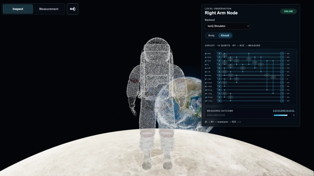Entangled BodyChanhyuk Park & Luke Shim · u/lukeshim · Python + QiskitEntangled Body is an interactive 3D artwork that treats the body as a network of 14 quantum nodes, each mapped to a specific body region.

Quantum Garden: correlated traits from one circuit

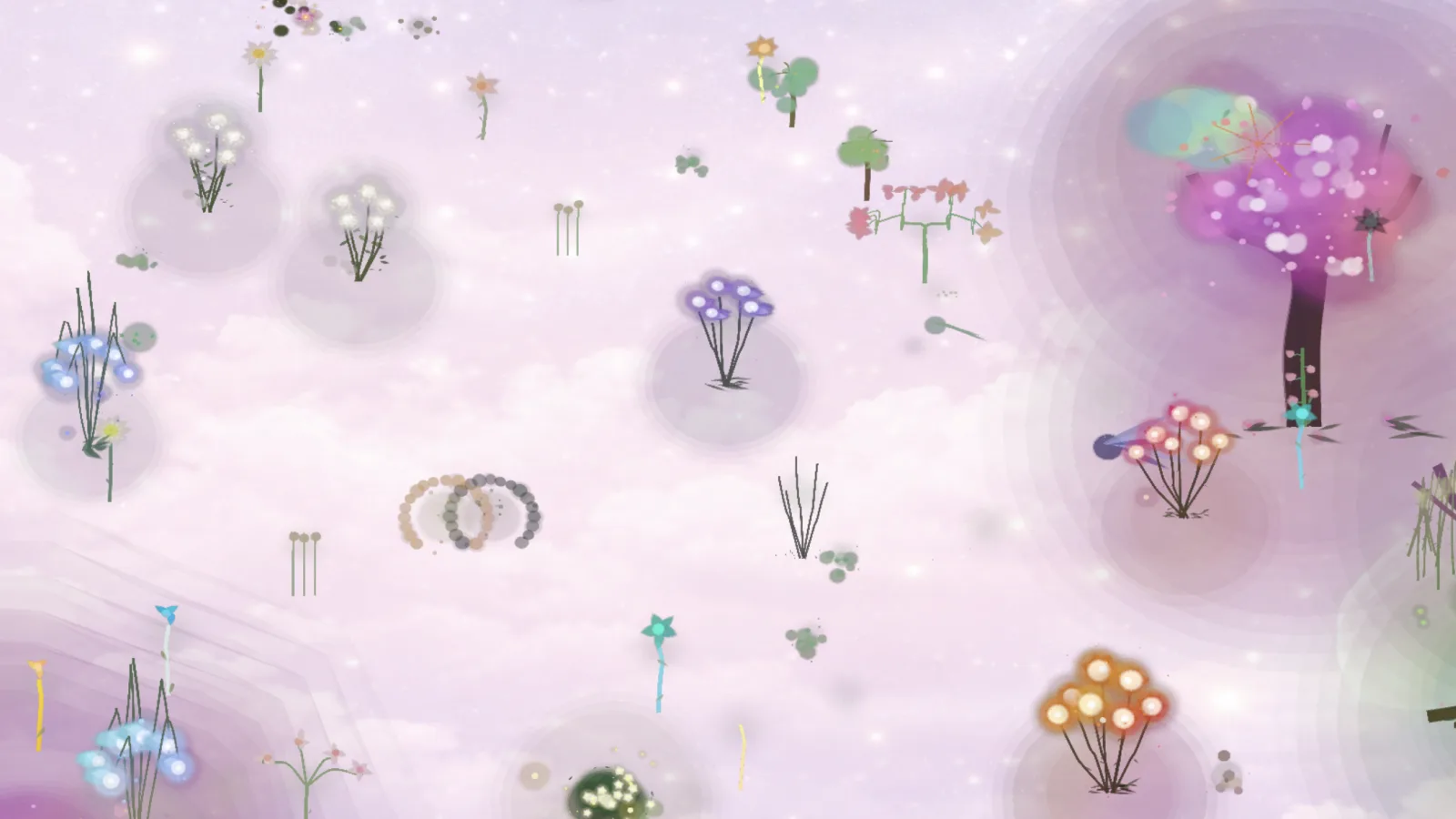
Quantum Garden draws each plant's traits from a precomputed pool of quantum measurement outcomes. Its rarest plants use the circuit below, which entangles five qubits so a plant's traits come out correlated with each other.

The garden also mirrors traits between plants in the same entanglement group, wherever they stand. The circuit does not reach across plants; the mirroring comes from the group sharing one stored result.

The circuit has six layers. A Hadamard on every qubit makes all thirty-two outcomes possible, seed-based rotations bias each qubit toward the plant's own tendencies, and a chain of CNOTs ties neighbours together.

Phase rotations follow, a second set of CNOTs couples qubits across the chain, and a last round of rotations sets the final state before measurement. Five measured bits come out, and every trait the plant shows is read off them.

None of the circuit runs while you watch. The project describes generating a pool of 500 results on IonQ ahead of time; hovering a plant assigns it one of those results and fixes its traits, and its group's, from then on.

​# Layer 3: Linear entanglement chain — correlates neighboring qubits
​for i in range(4):
1    circuit.cx(i, i + 1)
​​
​# Layer 4: Seed-based Rz phases — creates interference patterns
​# ...
​​
​# Layer 5: Cross-entanglement — non-local correlations across the circuit
​circuit.cx(0, 2)
​circuit.cx(1, 3)
2circuit.cx(2, 4)
1Four CNOTs in a row: 0 to 1, 1 to 2, 2 to 3, 3 to 4. Each ties a qubit to its neighbour, so the five bits stop being five independent coin flips.
2These three skip a neighbour. The chain already carried correlation past adjacent pairs, so they add direct long-range couplings instead of creating the first ones.

Fork Quantum Garden and delete the three cross-chain CNOTs. The neighbour chain still entangles the qubits, but the output distribution changes. Run both versions and compare which pairs of bits still move together. Mutual information, how much one bit's outcome tells you about another's, puts a number on it: on an exact simulation at the file's seed, for bits 2 and 3 it drops from about 0.25 bits with the cross CNOTs to 0.03 without them. Estimating it from counts takes about 1,000 shots; the file's default of 100, with its low-count filter, scatters too widely to show it.

Quantum GardenAmber Wang & Justin Pincar · u/AmberPincar · Python + QiskitQuantum Garden is an interactive generative art installation where digital plants exist in quantum superposition until observed.

Quantum Patterns: entanglement that spreads across a grid

Quantum Patterns runs a grid of cells and updates every one with the same small circuit. The cells overlap, so whatever that circuit does to its two qubits does not stay in one cell. Entangle them and the correlation spreads across the grid.

The project is a partitioned quantum cellular automaton: a grid that updates in steps, every cell by the same rule. The grid is cut into two-qubit cells in two ways, offset by one qubit, and both cuts are applied one after the other inside every step, so a cell's right qubit is a neighbouring cell's left qubit before the step is over.

The quickstart's cell circuit is a single CNOT on a grid that starts with one qubit set to 1 at the left edge. On its own that is a classical, reversible rule: it moves bits around and creates neither superposition nor entanglement. Treat the lone CNOT as the baseline.

​# The circuit applied to every cell. Here: a single CX on 2 qubits.
1cell = qiskit.QuantumCircuit(CELL_SIZE)
2cell.cx(0, 1)
​# Two offset tessellations make the update couple across cell borders.
3tes = pqca.tessellation.one_dimensional(NUM_QUBITS, CELL_SIZE)
1This small circuit is applied to every cell of the grid on every step.
2A single CNOT: on plain 0s and 1s it only shuffles bits around.
3This cuts the grid into two-qubit cells; the two offset cuts described above both run inside every step.

Putting cell.h(0) in front of cell.cx(0, 1) makes the rule quantum: the Hadamard creates superposition, the CNOT entangles the cell's two qubits, and because the cuts overlap, the entanglement does not stay inside one cell.

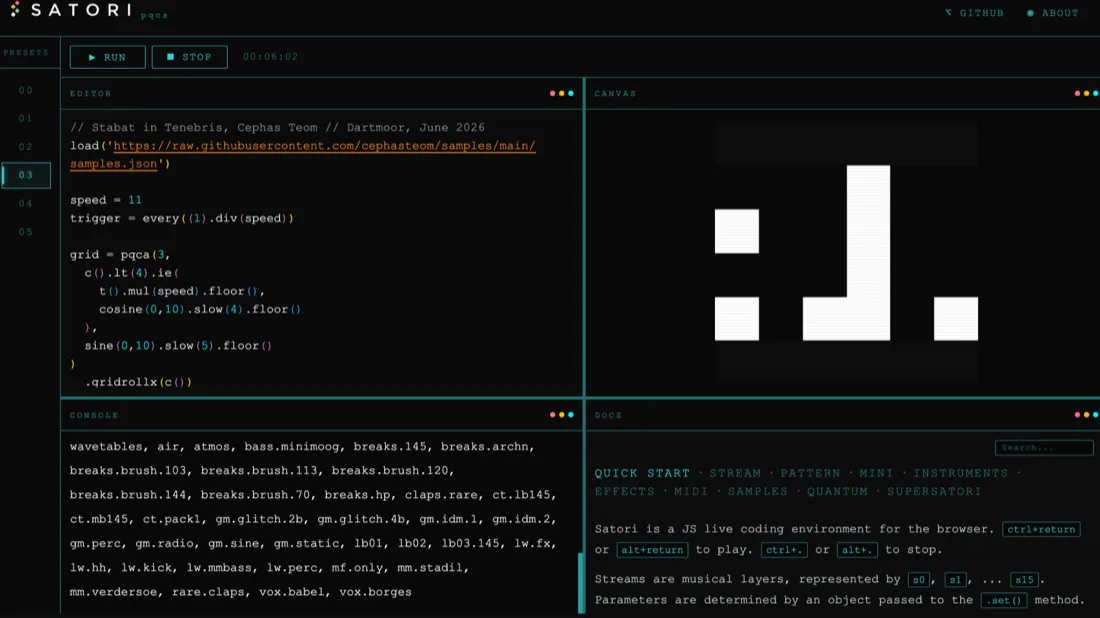Quantum PatternsPeter Thomas & Paulo Itaboraí · u/cephasteom · Python + QiskitQuantum Patterns explores Partitioned Quantum Cellular Automata (PQCA) as the basis for live-coded musical composition.

Quantum Butterfly Field: repairing a scrambled qubit

Quantum Butterfly Field scrambles five qubits together with random entangling gates until the state is spread across all of them, then damages one qubit. Running the scramble backwards recovers much of what that qubit held.

Five butterflies are five qubits. Each layer turns every qubit by two random angles, one about x and one about z, and then entangles two random pairs. After three layers part of what each butterfly held has moved into correlations with the others, more for some butterflies than for others. Then one butterfly is damaged: an extra qubit is coupled into it, which severs its correlations with the rest.

In a classical chaotic system that damage would be permanent, because small damage cascades (the butterfly effect). Once information is scrambled deeply enough across an entangled system, the correlations between the qubits hold it, so running the scramble backwards can recover much of the damaged qubit's state from the others.

Recovery is partial: on an exact simulation with the file's seed (42) and damaged qubit (qubit 2), the repaired qubit matches what it started as about 83% of the time. Yan and Sinitsyn showed the recovery in 2020, in a paper on recovering damaged information, and it is known as the quantum anti-butterfly effect.

Xinyi Zhang pairs the physics with lōkahi, the Native Hawaiian idea of wholeness through relationship.

The project's score is built from the length of the repaired qubit's Bloch vector, so it measures how sharply defined that qubit ended up. Whether the qubit came back as the state it started in is a separate check.

​# Random disjoint CX pairs: shuffle all qubits, pair them up.
​qubits = list(range(n_qubits))
1rng.shuffle(qubits)
2for i in range(0, n_qubits - 1, 2):
3    layer.append(('cx', int(qubits[i]), int(qubits[i + 1])))
1Shuffle the five qubits into a random order, so each layer draws its own pairing rather than reusing one.
2Step through them two at a time. Five qubits gives two pairs, with one left out of this layer.
3One CNOT per pair.

Fork the Butterfly Field and set N_LAYERS in main() to 1, then 2, then 3.

The score does not climb steadily: on an exact simulation with the same seed it lands near 0.79, 0.67 and 0.79, and other seeds land elsewhere. For that check, compare the repaired qubit against the state it was prepared in instead of against the length of its Bloch vector.

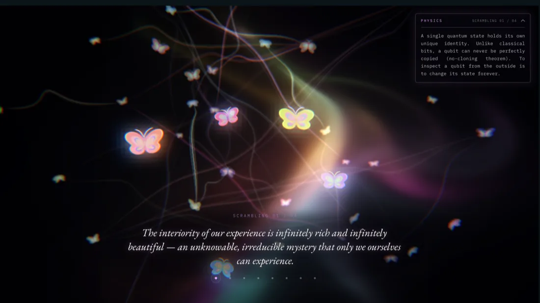Quantum Butterfly FieldXinyi Zhang · u/xinyi · Python + QiskitQuantum Butterfly Field is an interactive artwork bridging quantum computing concepts with indigenous epistemologies to explore repair and resilience in an interconnected world.

More than two qubits

Two qubits is the smallest case. With more, they can all share one state, a GHZ state, where every qubit comes out 0 together or 1 together:

​from qiskit import QuantumCircuit
​​
​n = 5
1qc = QuantumCircuit(n, n)
2qc.h(0)
​for i in range(n - 1):
3    qc.cx(i, i + 1)
4qc.measure(range(n), range(n))
​job = backend.run(qc, shots=1000)
5print(job.result().get_counts())
1Five qubits this time, and five ordinary bits to read them into.
2Put the first qubit into superposition, exactly as in the Bell state.
3Then pass it along the line: 0 entangles 1, 1 entangles 2, and so on to the end.
4Measure all five at once. range(n) is qubits 0 to 4, read into bits 0 to 4.
5On a noise-free simulator only two keys appear: all five qubits read 0 together or 1 together.

In a GHZ state, measuring any one qubit decides the other four, and losing one leaves the other four in a classical mixture. Error correction and precision sensing build on its correlations.

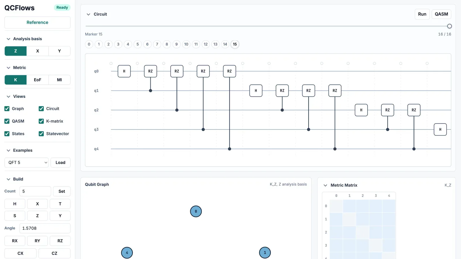
You can work out pair correlations from the counts by hand, but only in the basis you measured, and doing that for a whole circuit takes time. QCFlows, a correlation viewer by Paulo Itaboraí, Iosifina Angelidi and Kostas Blekos, draws a circuit's correlations directly as a graph: run a GHZ state through it and every qubit links to every other.

Entanglement on real hardware

An exact simulator such as Qiskit's Statevector holds the state as its list of numbers and returns all of them, entanglement included. The 2-qubit visualiser draws its pictures from such a state, which a quantum computer never lets you read. Every backend in the Playground, simulators included, returns counts, the same as hardware.

Hardware gives you counts and nothing else, so the Bell state example ends by computing two percentages and a threshold check from them.

1correlated = counts.get("00", 0) + counts.get("11", 0)
2uncorrelated = counts.get("01", 0) + counts.get("10", 0)
​print(f"\nCorrelated (|00⟩+|11⟩): {100*correlated/shots:.1f}%")
​print(f"Uncorrelated (|01⟩+|10⟩): {100*uncorrelated/shots:.1f}%")
​​
3if correlated / shots > 0.95:
​    print("✓ Strong entanglement confirmed!")
​else:
​    print("⚠ Noise detected — some uncorrelated outcomes")
1The two outcomes a Bell state is allowed to produce.
2The two outcomes it cannot produce. On an ideal simulator this is always zero.
3The threshold is picked by hand. Below it, more than 5% of the shots landed in the two outcomes a Bell state cannot produce, which this example treats as too noisy.

The threshold is a noise reading: 01 and 10 are impossible for a Bell state, so every shot that lands there came from the device, and the percentage measures that noise. It does not establish entanglement, because a pair of gloves clears 95% correlated as easily as a Bell pair does, and a single basis cannot separate the two. Confirming entanglement takes the second-basis test, which is another job on the machine.

An ideal simulator gives you a flawless Bell pair every time, so it cannot tell you how much entanglement is left on a device by the time the circuit ends. A GHZ state across five qubits is a standard test for that, because noise on any one of its qubits weakens the correlations of all five.

Start with two qubits

Each project on this page puts an entangling operation on its qubits, or would with one added gate, and each project's measurement shows a different amount of the resulting entanglement.

The Bell state is the smallest version, two gates and a measurement, and the second-basis test separates it from a pair of gloves.