Understanding Quantum Interference
Amplitudes carry signs, so they can reinforce or cancel. How the cancellation works on one qubit, in Grover's search and in three community projects.

About the author
Quantum interference lets a circuit move probability onto some outcomes and away from others. Superposition alone does not: a qubit in an equal superposition measured a thousand times gives roughly five hundred 0s and five hundred 1s, the same split as a thousand coin flips.
What is quantum interference?
Quantum interference happens when a circuit can reach the same outcome by more than one route. Every route carries an amplitude, a number with a size and a direction, and the simplest useful case is an amplitude that is either positive or negative. The routes leading to one outcome are added together, and the probability comes from the size of that sum. Routes that point the same way reinforce each other, and a positive and a negative route of the same size cancel to zero.
Grover's search uses cancellation between routes to raise a one-in-eight guess to a 94.5% hit rate in two iterations.
Where interference came from
Interference was observed in light long before anyone built a qubit, and since then in electrons and in molecules.
At Young's bright fringes the light from the two sides of the card arrives in step, and the two contributions add. Each dark band is a place that light can reach by either route but where little or none arrives, and blocking one of the two routes makes it brighter: the second route subtracts from the first.
Each experiment in the timeline gives the light or the particles more than one route to the screen.
Taylor's fringes came out as sharp as with a bright lamp, so the pattern does not come from photons interacting with each other. In Tonomura's film the pattern builds up from single electrons over about twenty minutes.
Adding amplitudes before squaring
A quantum state carries an amplitude for each outcome. Squaring an amplitude's size gives the probability of that outcome, so a negative amplitude and a positive one of the same size are equally likely to be measured. When two routes lead to the same outcome their amplitudes are added first, and the squaring happens to the sum. Feynman's Lectures on Physics introduce the rule with the two-slit experiment.
Classical probabilities for separate routes can only add: two routes to the same outcome, each with a one-in-four chance, give a one-in-two chance of getting there. Two positive numbers do not add to zero, so Young's dark bands cannot come from adding probabilities.
Take two routes with amplitudes of +0.5 and −0.5. Add the two amplitudes and the sum is 0, and 0 squared is 0, so the outcome never happens. Square each amplitude first and each route gives 0.25, and 0.25 plus 0.25 is 0.5, so the outcome happens half the time.
Cancelling in one place does not remove probability from the pattern as a whole, which always totals one. The probability missing from a dark band turns up at the bright bands, so a bright band is brighter than either route produces alone.
The smallest cancellation you can make
A circuit version of Young's experiment takes three gates. A Hadamard opens two routes, an rz sets how far out of step they are, and a second Hadamard brings them back together, where they add or cancel.
# 'backend' is pre-created for you in the Qollab Playground.
from math import pi
from qiskit import QuantumCircuit
def zeros(theta):
qc = QuantumCircuit(1, 1)
1 qc.h(0)
2 qc.rz(theta, 0)
3 qc.h(0)
qc.measure(0, 0)
counts = backend.run(qc, shots=1000).result().get_counts()
4 return counts.get('0', 0)
for name, theta in [("0", 0), ("pi/4", pi / 4), ("pi/2", pi / 2), ("3pi/4", 3 * pi / 4), ("pi", pi)]:
5 print(f"rz({name:>5}) -> {zeros(theta)} zeros out of 1000")
- 1After one Hadamard the qubit has two routes open, the
0 route and the 1 route, and measuring here gives roughly 500 of each. - 2Turn a phase on the
1 route. The rz moves no probability: measure right after this line and the tally is still about 500 each, whatever the angle. - 3The second Hadamard sends both routes to both answers, so each answer is reached twice, and the two contributions add or cancel according to the angle.
- 4How many of the thousand shots read
0. - 5Five jobs at five angles: the count of
0s falls from 1000 to 0, and only the phase changes.
rz angle | shots reading 0 |
|---|---|
| 0 | 1000 |
| π/4 | ~854 |
| π/2 | ~500 |
| 3π/4 | ~146 |
| π | 0 |
To run the listing, paste it into a Playground project and choose the Built-in simulator, the first entry under Locally Run Simulators in the Run on Qollab dialog. The listing sends five jobs, one per angle, and on an IonQ backend the Playground allows one job per run of your code. The IBM entries in the same group add a device's noise, so on those the top and bottom rows come out near 1000 and 0.
The expected number of 0s is 1000 × cos²(θ/2). The top and bottom rows use the same three gates and the same measurement, and one gives 0 with certainty while the other gives 1.
random.randint(0, 1) gives you the middle row. A classical random draw can be biased, but two classical probabilities cannot cancel, because a probability has no sign.
The second Hadamard is the circuit's screen: the qubit reaches 0 along both routes, the two amplitudes are added there, and θ sets whether they reinforce or cancel. At θ = π the two amplitudes cancel exactly, and all thousand shots land on 1.
The gates in these circuits
Five gates cover most of the excerpts on this page.
Hadamard
Takes a qubit sitting at 0 and leaves it with no fixed value: measure it and you get 0 or 1 with equal probability.
The Hadamard is its own inverse. Many circuits here start and end with a layer of Hadamards: the first opens the routes, the second recombines them, and the gates in between decide how they add.
Rotates the phase. The angle comes before the qubit, and it shifts the 1 half of the state out of step with the 0 half by that much; at π that is a flipped sign, and smaller angles go part of the way.
An rz on its own changes no probability: the counts are the same whether the angle is 0 or π, and the difference shows only after another gate recombines the two halves.
Controlled-Z
Flips the sign of one outcome, the one where both qubits read 1, and leaves the other three alone. Like rz it moves no probability by itself.
For more than two qubits the same job is written as h, a multi-controlled x, then h again on the last qubit. Both Grover circuits below write the flip that way, and Qiskit calls the three-qubit version of that x a ccx.
Swaps 0 and 1 on a single qubit, like a classical NOT.
In these circuits, x gates select which outcome gets a sign flip: wrap a cz in x gates and the flip applies to the outcome you choose.
Reads a qubit into an ordinary bit and forces it to a definite 0 or 1. Measurement cannot be undone, and the sign of an amplitude never appears in its counts.
So every circuit here has to turn its signs into probabilities before this line.
Grover's search: a mark that changes none of the odds
Qollab ships a runnable Grover's search. Three qubits give eight possible answers, one of which is the target, and a Hadamard on each qubit starts all eight at 12.5%.
The first half of the algorithm is the oracle, which marks the target.
target = "101"
# ...
# ── Oracle: phase-flip the target state ──────────────────────────────
def build_oracle(target):
n = len(target)
oracle = QuantumCircuit(n, name="Oracle")
for i, bit in enumerate(reversed(target)):
if bit == "0":
1 oracle.x(i)
if n == 2:
oracle.cz(0, 1)
elif n == 3:
oracle.h(2)
2 oracle.ccx(0, 1, 2)
oracle.h(2)
else:
oracle.h(n - 1)
oracle.mcx(list(range(n - 1)), n - 1)
oracle.h(n - 1)
for i, bit in enumerate(reversed(target)):
if bit == "0":
3 oracle.x(i)
return oracle
- 1These
x gates select which outcome the flip below applies to. 101 has a 0 in the middle, so the middle qubit gets flipped and the answer being marked temporarily becomes 111. - 2These three lines are the mark:
h, ccx, h together flip the sign of the one outcome where all three qubits read 1, so one of eight amplitudes becomes negative and the other seven are untouched. - 3Undo those
x flips, so the sign now sits on 101, the target.
The function as a whole moves no probability: run it on the eight-way superposition and all eight outcomes still sit at 12.5%.
The mark is a sign, which a measurement cannot report, like the phase the rz wrote in the one-qubit listing.
Turning the mark into probability
The second half of Grover's search is the diffuser, the same h, phase, h arrangement on three qubits.
# ── Diffuser: amplify the marked state ───────────────────────────────
def build_diffuser(n):
diffuser = QuantumCircuit(n, name="Diffuser")
1 diffuser.h(range(n))
diffuser.x(range(n))
if n == 2:
diffuser.cz(0, 1)
elif n == 3:
diffuser.h(2)
2 diffuser.ccx(0, 1, 2)
diffuser.h(2)
else:
diffuser.h(n - 1)
diffuser.mcx(list(range(n - 1)), n - 1)
diffuser.h(n - 1)
diffuser.x(range(n))
3 diffuser.h(range(n))
return diffuser
- 1Recombine the routes, the same move as the second Hadamard in the one-qubit listing, on all three qubits at once.
- 2The same sign flip as the oracle, which the
x layer applies to the all-zeros outcome this time. The diffuser is the same for every target; only the oracle depends on it. - 3After the closing Hadamard layer, every amplitude is the same distance from the average as before, on the other side of it, so the one the oracle pushed below the average ends up furthest above it.
The standard name for those seven lines is inversion about the mean. In the first iteration, seven amplitudes are positive and one is negative, so the average sits below the positive ones. Reflecting each amplitude through that average takes the negative one from −0.35 to about +0.88 and halves each of the other seven, from 0.35 to about 0.18. The project's diffuser also flips every sign at once, so a statevector of its circuit shows −0.88 and −0.18; a sign shared by every amplitude changes no count.
Run the oracle and the diffuser as a pair and the chance of measuring 101 moves like this.
| Grover iterations | chance of reading 101 |
|---|---|
| 0 | 12.5% |
| 1 | 78.1% |
| 2 | 94.5% |
| 3 | 33.0% |
Two iterations, and so two calls to the oracle, take a one-in-eight guess to a 94.5% hit rate. A classical scan that checks the eight items one by one until it finds the target takes 4.5 checks on average.
Too many iterations undo the answer
After three iterations the target is back down to 33.0%. The project computes how many iterations to run from the size of the search space.
target = "101"
shots = 1000
num_qubits = len(target)
1num_iterations = int(math.pi / 4 * math.sqrt(2 ** num_qubits))
- 1For three qubits this works out at 2.221, and
int takes it down to 2. The formula is π/4 times the square root of the search space, and that square-root growth is Grover's quadratic speedup.
Each iteration turns the state by a fixed angle toward the marked answer and keeps turning past it: after the peak, the same interference spreads the probability out again.
Try this when you fork it. Replace num_iterations with 3 and run. The target falls from 94.5% to about a third, and a fourth iteration takes it to roughly 1%, worse than the 12.5% you started with.
Quantum Advantage Lab: a quantum walk
Quantum Advantage Lab's third race compares a quantum walk with a classical random walk, both in the same repository. Interference in the quantum walk shapes the whole distribution of where the walker ends up.
A classical random walker starts at node 0 and picks a neighbour at each step. By default the race runs a thousand walkers.
# For each walker, pick next position based on transition probabilities
new_positions = np.empty(n_trials, dtype=int)
for trial_idx in range(n_trials):
current = positions[trial_idx]
new_positions[trial_idx] = rng.choice(
n_nodes, p=transition[current]
1 )
positions = new_positions
# Build empirical distribution
counts = np.bincount(positions, minlength=n_nodes)
2 distribution = (counts / n_trials).tolist()
- 1Each walker makes a fresh random draw on every step, so the race's defaults of a thousand walkers and ten steps come to ten thousand draws.
- 2Tally where the thousand walkers ended up. Around the ring the tally is a bell curve centred on the start; the Lab's chart puts the start at its left edge, so the two halves of the bell sit at the chart's two ends.
The quantum walk draws no random number at any step. The walk turns a coin qubit and shifts the walker according to the coin, both as ordinary gates, and nothing is sampled until the finished circuit is measured.
# Initial state: walker at position 0, coin in superposition
if graph_type == "cycle":
1 qc.h(coin_qubits[0])
# ...
for step in range(n_steps):
# Coin
if graph_type == "cycle":
2 _hadamard_coin(qc, coin_qubits[0])
# ...
# Shift
if graph_type == "cycle":
3 _cycle_shift(qc, coin_qubits[0], position_qubits)
- 1The Hadamard leaves the coin with no fixed value, and nothing in the walk measures it.
- 2Each step turns the coin again with another Hadamard, and the walk keeps every route open.
- 3Move the walker according to the coin, both ways at once. The position register is a superposition over every node the walker could have reached, held open until the final measurement.
Ten steps in, the classical walker has taken one of 1,024 routes and the tally counts how often each endpoint came up. The quantum walk samples none of them: the amplitudes of routes that reach the same node are added, and routes that arrive out of step cancel before anything is counted.
The quantum walk's distribution is not a bell curve: cancellation leaves it lopsided and ridged. On a ring big enough that routes going round in opposite directions have not yet met, the distribution also widens in proportion to the number of steps, where the classical walk widens with the square root.
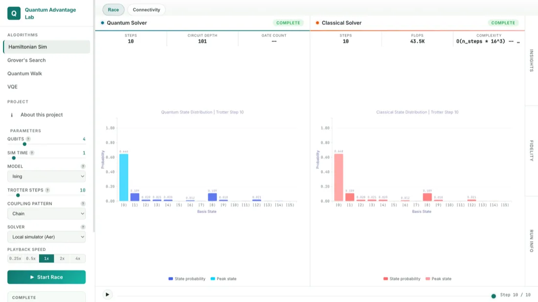 Quantum Advantage LabReal-time interactive platform that races four foundational quantum algorithms against their classical counterparts, visualizing each solver's progress step by step.
Quantum Regime Radar: running a circuit backwards to compare two states
Quantum Regime Radar scores a market window, such as NVDA's 2022 returns, against five volatility regimes taken from past market episodes, each one encoded as a twelve-qubit state. Scoring means comparing two states, and neither state can be read.
The project builds one state, then runs the other's circuit in reverse and counts how many shots return to all-zeros.
def _inversion(qc_live: QuantumCircuit, qc_ref: QuantumCircuit) -> QuantumCircuit:
n = qc_live.num_qubits
qc = QuantumCircuit(n, n)
1 qc.compose(qc_live, inplace=True)
2 qc.compose(qc_ref.inverse(), inplace=True)
qc.measure(range(n), range(n))
return qc
- 1Prepare the market window's twelve-qubit state.
- 2Then append the inverse of the reference regime's circuit: the same gates in reverse order, each one reversed, which undoes the preparation of the reference state exactly.
Four thousand and ninety-six outcomes are possible on twelve qubits, and every one of them is reached by many routes through the two circuits. If the window's state and the reference are the same, the inverse cancels the preparation and every route recombines on all-zeros. If the two states differ, the cancellation is partial and shots land on other bitstrings.
So the fraction of shots reading all zeros estimates the squared overlap between the two states, measured without either state being inspected.
live = _build(DEMO_PARAMS[ci][REF_FAM[target]])
ref = _build(REF_PARAMS[target])
circuit = transpile(_inversion(live, ref), backend=backend, optimization_level=0)
1 result = backend.run(circuit, shots=shots).result()
counts = result.get_counts()
if isinstance(counts, list): # defensive; single circuit expected
counts = counts[0]
2 K_meas = _zero_frac(counts)
3 sigma = (K_meas * (1.0 - K_meas) / max(shots, 1)) ** 0.5
- 1On IonQ backends the Playground allows one job per run, so this cell spends it on one comparison.
- 2The kernel is the fraction of all-zero shots.
- 3Its error bar: the standard error of a fraction estimated from
shots samples.
The inversion test has the shape of the one-qubit listing, prepare then undo, with a second circuit doing the undoing.
Quantum Regime RadarScores live equity returns against five volatility regimes taken from real market history, using quantum kernels on IonQ.Musiq: a phase on every qubit at once
Musiq turns a circuit into sound. One of Musiq's generators maps the phase of each statevector amplitude onto the phase of an oscillator.
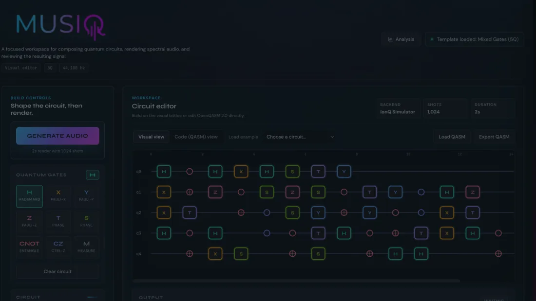
Musiq's waveform generator, which turns measured counts into sound, includes an IQP builder with the same shape as the Grover diffuser.
n = self.n_qubits
# n diagonal Rz params + (n-1)+(n-2) CZ layer = n + 2*n-3 for two CZ "bands"
num_rz = n
params = ParameterVector("λ", num_rz)
qc = QuantumCircuit(n)
1 qc.h(range(n))
for qubit in range(n):
2 qc.rz(params[qubit], qubit)
# Fixed CZ pattern (nearest-neighbor style, no random choice)
for i in range(n):
for j in range(i + 1, min(i + 3, n)):
3 qc.cz(i, j)
4 qc.h(range(n))
qc.measure_all()
- 1Open every route at once. At the waveform generator's default of eight qubits that is 256 outcomes, all equally likely at this line.
- 2One phase per qubit, with the parameters named λ; none of these angles changes a probability.
- 3The
cz gates add phases between pairs of qubits, on top of the per-qubit ones, and every outcome is still equally likely going into the next line. - 4The closing Hadamard layer recombines every route: the phases written above decide where routes reinforce and where they cancel, and the equal probabilities become a distribution shaped by those angles.
IQP stands for instantaneous quantum polynomial time. Everything between the two Hadamard layers is diagonal, so every gate there only writes phases.
Musiq's waveform generator draws the λ angles at random each time it builds this circuit, so each build gives a different distribution and a different spectrum.
MusiqMusiq is a browser-based quantum sonification platform that transforms quantum-circuit outputs into generative audio.Interference on noisy hardware
Interference needs the relative phase between two routes to survive from the gate that writes it to the gate that converts it, and on hardware, noise degrades phases as the circuit runs.
Deeper circuits give noise more time to degrade the phases. One iteration is an oracle and a diffuser, each with a multi-controlled sign flip that hardware does not have as a single operation. Transpiled for hardware, each flip becomes a run of two-qubit gates, and the three-qubit search is tens of operations deep by its second iteration.
The Grover's search project checks its own result at the end.
target_count = counts.get(target, 0)
success_rate = target_count / shots
print(f"\nTarget |{target}⟩ found: {target_count}/{shots} ({100*success_rate:.1f}%)")
1print(f"Classical random guess would give: {100/2**num_qubits:.1f}%")
# ...
2if success_rate > 0.8:
print("✓ Grover's search successful!")
else:
print("⚠ Lower than expected — noise may be affecting results")
- 1This prints 12.5%, what a uniform random guess scores; the circuit has to beat that for its interference to show in the counts.
- 2The threshold is picked by hand, well below the 94.5% the maths predicts, to allow for gate and readout error and the scatter of a thousand shots.
None of these circuits is faster than a laptop. Eight items is a trivial search, and a classical computer checks all of them before an IonQ job has left the queue. Grover's advantage is quadratic and it needs a search space far larger than anything a current device can hold with its phases intact.
A hardware run shows what noise does to the result. An ideal simulator matches the predicted 94.5% up to shot noise, so the gap between that figure and the success rate on hardware is the combined effect of gate and readout errors.
Quantum Advantage Lab caches its hardware runs in its repository and replays them, so a race can show a hardware result without queuing the same job again.
Start with Grover
Every circuit on this page relies on signs or phases that a measurement cannot see, until a later gate recombines the routes. In Grover's search the oracle writes the sign, and the diffuser turns it into counts.
Fork Grover's search first: it runs in the Playground with no setup, and the oracle and the diffuser are under forty lines together.
Run it, then move the target.
Fork Grover's search, run it as shipped, and run it again with target set to another of the eight bitstrings. Then open any project above and find the line where its phases turn back into counts.
Stay in the loop.
Get the latest tutorials, demos, and project showcases straight to your inbox. No noise, just the good stuff.
Enable JavaScript to sign up.
Qollab updates only. Unsubscribe any time. Privacy Policy.
- 1About the author
- 2What is quantum interference?
- 3Where interference came from
- 4Adding amplitudes before squaring
- 5The smallest cancellation you can make
- 6The gates in these circuits
- 7Grover's search: a mark that changes none of the odds
- 8Turning the mark into probability
- 9Quantum Advantage Lab: a quantum walk
- 10Quantum Regime Radar: running a circuit backwards to compare two states
- 11Musiq: a phase on every qubit at once
- 12Interference on noisy hardware
- 13Start with Grover