Understanding Quantum Measurement
Why one shot says little about the odds, why the basis you measure in changes the answer, and how readout errors get corrected.

About the author
Measurement is the only way to get anything out of a qubit, and it hands you a single 0 or 1. There is no print(qubit) and no way to step through a circuit and watch a qubit change.
Measurement produces that 0 or 1 instead of finding it: before you measure, the qubit holds no answer to print. So you write a program, run it, get back a tally of bitstrings, and infer what you wanted to know from that tally.
Four consequences follow: you can sample a qubit but never read it, the answer depends on which question you ask, measuring is one-way and erases whatever the qubit held, and the instrument doing the measuring can make errors of its own.
The smallest measurement you can make
One qubit is enough: put it into a state that has no fixed value, measure it, and count what comes back.
# 'backend' is pre-created for you in the Qollab Playground.
from qiskit import QuantumCircuit
1qc = QuantumCircuit(1, 1)
2qc.h(0)
3qc.measure(0, 0)
4one = backend.run(qc, shots=1).result().get_counts()
5many = backend.run(qc, shots=1000).result().get_counts()
print(one, many)
- 1One qubit to do the quantum work, and one ordinary bit to read the answer into.
- 2A Hadamard puts the qubit into superposition. It has no value to read until it is measured.
- 3The measurement forces the qubit to one definite answer and writes that answer to the bit.
- 4Run the circuit for one shot. You get
{'0': 1} or {'1': 1}: one answer, with nothing to say whether the other was equally likely or nearly impossible. - 5Run it for a thousand shots. Now the pattern shows: roughly 500 each. A shot is one execution of the circuit, and the odds only show across many shots.
The listing sends two jobs, and on an IonQ backend the Playground allows one job per run of your code, so run it on the Built-in simulator, the first entry under Locally Run Simulators in the Run on Qollab dialog.
The qubit held something before qc.measure, the measurement turned it into a 0 or a 1, and what it held cannot be recovered from the result. Run the same program twice and the thousand-shot tally comes back roughly the same, while the single shot can flip between runs, because it is a single sample.
Superposition is the word for what the qubit had before the measurement.
A run returns counts
A run on a quantum computer returns a dictionary mapping each bitstring to how many times it came up, and nothing else.
# Counts from an ideal Bell-state experiment: only correlated outcomes,
# roughly 50/50 between 00 and 11
1ideal = {"00": 512, "11": 488}
plot_histogram(ideal, filename="ideal.svg")
# The same experiment on noisy hardware leaks shots into 01 and 10.
# plot_histogram overlays multiple experiments for direct comparison.
2noisy = {"00": 462, "01": 27, "10": 31, "11": 480}
plot_histogram(
[ideal, noisy],
legend=["ideal simulator", "noisy device"],
filename="ideal_vs_noisy.svg",
3)
- 1A thousand shots of a Bell pair, as a tally of outcomes.
- 2Illustrative counts for the same circuit on noisy hardware:
01 and 10 should be impossible for this state, and here 58 shots out of a thousand land there. - 3
plot_histogram draws both tallies on one chart, so you can compare them.
The gates in these circuits
Four gates and one instruction cover every excerpt below.
Hadamard
Takes a qubit sitting at 0 and leaves it with no fixed value: measure it and you get 0 or 1 with equal probability.
The Hadamard is its own inverse: two in a row put the qubit back where it started.
Leaves a qubit exactly as likely to read 0 or 1 as it already was, and flips the sign in front of the 1 half of the state.
A measurement does not report the sign, so a z on its own does not change the counts.
Rotates a qubit by an angle. The angle comes before the qubit in the call and sets how likely a qubit starting at 0 is to read 1.
At 0 it is certain to read 0, at π certain to read 1, and at π/2 it gives the same even split the Hadamard does. Any angle in between sets a bias, so a circuit can have odds other than fifty-fifty.
Couples two qubits by an angle. Unlike the others it does not change how often either qubit reads 0 or 1.
The coupling shifts the phase of the pair's state by an amount that depends on whether the two qubits agree.
Reads a qubit into an ordinary bit and forces it to a definite 0 or 1. Measurement cannot be undone: whatever the qubit held before is gone once you look.
A single shot therefore gives one outcome and says little about the odds behind it, so the circuits here are run many times over.
The basis: which question you ask
Measuring puts a question to the qubit, and 0-or-1 is only one of the questions available. To see that, build two qubit states that give the same counts, and then ask them something else.
# 'backend' is pre-created for you in the Qollab Playground.
from qiskit import QuantumCircuit
def counts(add_z, ask_after_h):
qc = QuantumCircuit(1, 1)
1 qc.h(0)
if add_z:
2 qc.z(0)
if ask_after_h:
3 qc.h(0)
qc.measure(0, 0)
return backend.run(qc, shots=1000).result().get_counts()
4print("h asked directly :", counts(False, False))
5print("h,z asked directly :", counts(True, False))
6print("h asked after an h:", counts(False, True))
7print("h,z asked after an h:", counts(True, True))
- 1Both states start the same way, with the Hadamard from the first listing.
- 2This
z is the only difference between the two states. It leaves the qubit as undecided as it was and flips the sign in front of the 1 half. - 3This Hadamard is not part of the state: it comes after the state is prepared, right before the measurement, and switching it on changes the question.
- 4Roughly 500 each, the same even split as the first listing.
- 5Roughly 500 each again. Nothing in this tally can tell the two states apart.
- 6Every shot reads
0. Two Hadamards cancel, so the qubit is back where it started. - 7Every shot reads
1. The same two states as the rows above, and now the answers are opposites.
| prepared with | asked directly | asked after an h |
|---|---|---|
h | ~500 0, ~500 1 | 1000 0 |
h then z | ~500 0, ~500 1 | 1000 1 |
The z changed the qubit, and the direct question could not report the change.
The question is called a basis: measuring directly asks in one basis, and a Hadamard before the measurement switches to another. The state is the same in both columns. No single basis reports everything about a state, and measuring in the wrong one can leave the part your circuit worked on out of the output, with nothing in the output to say so.
Each of the four printed lines needed its own run and a fresh qubit, so the listing sends four jobs and also needs the Built-in simulator. The measurement is the last line of the function every time, because you cannot ask one question, look, and then ask the other: the state is gone after the first.
On real hardware the right-hand column will not come back as a clean 1000 and 0: some shots land on the other outcome, because of gate and readout errors.
When the odds are not fifty-fifty
Every circuit so far has aimed at an even split or a certainty; Entangled Body needs odds in between.
Entangled Body is a 3D human figure whose fourteen regions are fourteen qubits. Touch one and the figure responds around it, strongly nearby and less further away.
Each region needs its own probability of lighting up, and the piece has a two-line function that turns a probability into an Ry angle.
def _prob_to_ry(prob):
1 p = max(0.0, min(1.0, prob))
2 return 2.0 * asin(sqrt(p))
- 1Hold the requested probability between 0 and 1, so a rounding error upstream cannot ask for odds that do not exist.
- 2Turn it into an Ry angle: name the odds you want and this returns the rotation that produces them.
The conversion is exact: ask for 0.84 and the odds of reading 1 are 0.84.
Entangled Body uses that to draw its ripple. A hover sets the region you touched to a certainty, its nearest neighbour to between about 0.97 and 0.98, depending on where you touch, and the furthest region to 0.90.
In a single shot most or all regions read 1, so one shot shows no ripple. Across the 1024 shots the project runs, the nearest region reads 0 about 20 to 30 times and the furthest about a hundred.
On top of the rotations, the anatomical links between regions get an rzz coupling, and those entangle the state. They also leave no trace in the counts: an rzz only shifts phases, and the circuit measures directly, in the basis where phases do not show.
Fork Entangled Body and put a Hadamard on every region before the measurement, the same move as the right-hand column of the table above. The couplings then change the counts: every coupled region except the one you touched, which a hover holds at certainty, shifts its odds of reading 1, by up to about a fifth on a hover.
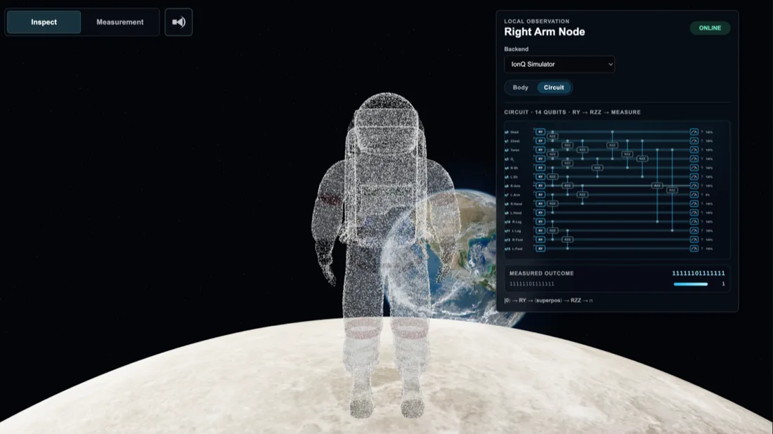 Entangled BodyEntangled Body is an interactive 3D artwork that treats the body as a network of 14 quantum nodes, each mapped to a specific body region.
Readout errors: when the instrument is wrong
A readout error leaves the state alone and gets the record wrong: the detector reports 1 when the qubit was 0, or 0 when it was 1. Because the error happens after the quantum part is over, ordinary arithmetic can undo it.
function qubitMatrix(q){
let p10=state.p10, p01=state.p01;
1 if(state.hotQubit && q===2){p10=Math.min(0.25,p10*4); p01=Math.min(0.25,p01*4);}
2 return [[1-p10,p01],[p10,1-p01]];
}
function Aentry(i,j){let p=1;
3 for(let q=0;q<N;q++){const bi=(i>>q)&1, bj=(j>>q)&1; p*=qubitMatrix(q)[bi][bj];}
return p;}
- 1One qubit can be worse than the others. On real devices readout quality varies from qubit to qubit and drifts over time.
- 2These four numbers are the whole error model for one qubit: how often a 0 is read as 0 or 1, and the same for a 1.
- 3Multiply the per-qubit numbers together to get the chance that the true bitstring j was recorded as i. Do that for every pair and you have a matrix describing the whole readout.
Build that matrix, and correcting the results is a linear algebra problem: you have the corrupted counts and the matrix that corrupted them, so you solve for what went in. The project does exactly that and shows three histograms side by side, ideal, raw and corrected.
Readout mitigationReadout error corrupts the measurement, not the quantum state - so classical math can undo it. Drag the error sliders on a GHZ-5 and watch three histograms (ideal, raw, corrected) update instantly.Musiq: hearing the distribution
Musiq turns a circuit's output into sound. Each run of the circuit brings a fresh tally of shots, so the music varies from run to run.
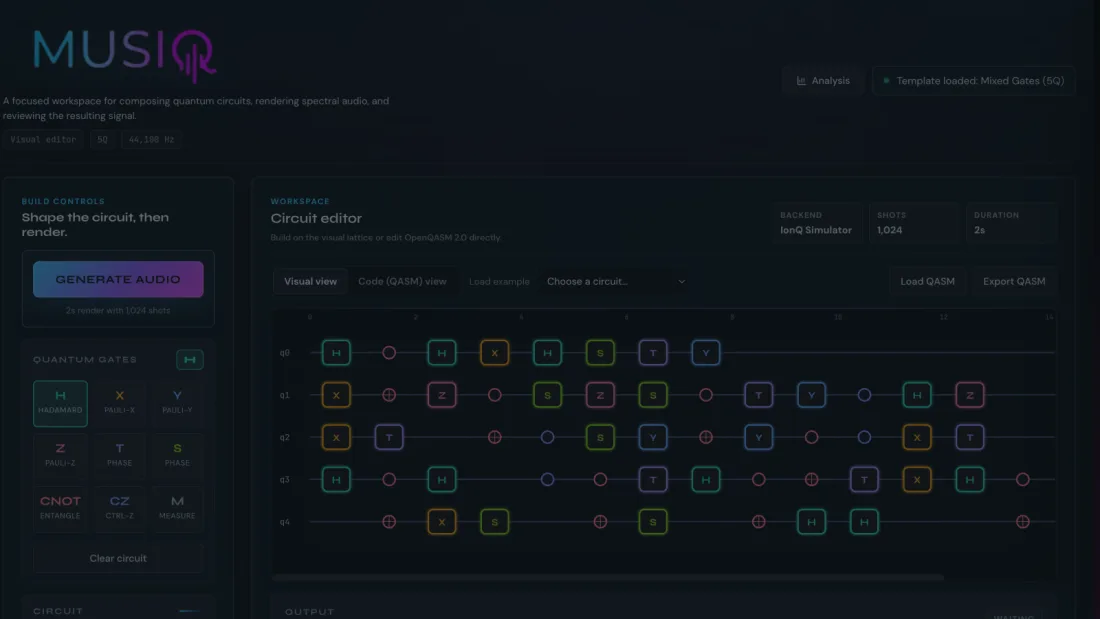
Musiq's mapper offers two methods in the same function: one plays the whole tally at once, and one plays it back one draw at a time.
if method == "weighted_sum":
for bitstring, prob in probability_dist.items():
1 if prob > 0.01:
amp = self.map_bitstring_to_amplitude(bitstring)
2 waveform += prob * amp
elif method == "stochastic":
# Probabilistic sampling from quantum outcome distribution
bitstrings = list(probability_dist.keys())
probs = np.array(list(probability_dist.values()))
probs = probs / np.sum(probs)
# Sample based on probability at each time point
for i in range(self.samples):
3 selected = np.random.choice(bitstrings, p=probs)
amp = self.map_bitstring_to_amplitude(selected)
waveform[i] = amp[i]
- 1Musiq's threshold: any outcome under one per cent is left out of the chord.
- 2Each remaining outcome is added in, scaled by its share of the shots, so you hear the whole tally at once, and the same tally always gives the same chord.
- 3The stochastic method draws one outcome per sample, weighted by the same shares, like shots, so it comes out different on every run.
The mapper's docstring calls the stochastic method sampling from "the quantum outcome distribution (not classical random generation)".
The one-per-cent threshold in the first branch is a judgement call: in a distribution, a rare outcome and a noise blip look the same, and the threshold drops both.
This listing comes from the project's repository rather than its Qollab page, which still carries the starter circuit.
MusiqMusiq is a browser-based quantum sonification platform that transforms quantum-circuit outputs into generative audio.Quantum Garden: one measurement per plant
Quantum Garden fixes each plant's traits from one stored measurement outcome.

The circuit behind a plant is fixed: each plant derives a seed from its own ID, and the same seed always builds the same five-qubit circuit.
seed = 42 # Each plant gets a deterministic seed from its ID hash
1circuit = QuantumCircuit(5, 5)
# Layer 1: Full superposition — all 32 outcomes initially possible
for i in range(5):
2 circuit.h(i)
# ...
# Measure all qubits
3circuit.measure([0, 1, 2, 3, 4], [0, 1, 2, 3, 4])
- 1Five qubits to do the work, and five ordinary bits to read the answers into. Five bits is thirty-two possible results.
- 2A Hadamard on each one, so all thirty-two start out equally likely. The five layers this excerpt skips then change the odds between them, and none of the thirty-two drops to zero.
- 3The measurement makes one draw from those odds: five bits, and every trait the plant shows is read off them.
The seed fixes the odds but not the outcome: simulate the finished circuit and all thirty-two outcomes still carry some probability, the likeliest only 22%. Run that identical circuit twice and about seven times in eight the second run gives you a different plant.
So a plant's traits come from its one draw; re-running the circuit would give a new one. The garden therefore stores each draw instead of recomputing it: the project describes generating 500 results on IonQ ahead of time, and a plant keeps the result it is given, so hovering again changes nothing.
Quantum GardenQuantum Garden is an interactive generative art installation where digital plants exist in quantum superposition until observed.QAVE: inspecting the state by simulating it
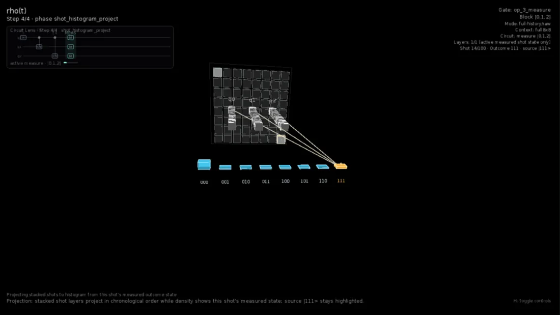
QAVE takes a Qiskit circuit and turns it into a deterministic trace: a frame-by-frame record of how the state evolves, which it then renders as an animation. To do that it needs the state, which a measurement destroys.
# Inspect the pre-measurement statevector
1pre_measurement = circuit.remove_final_measurements(inplace=False)
2psi = Statevector.from_instruction(pre_measurement)
print("Non-zero amplitudes before measurement (bitstring is |q2 q1 q0>):")
for basis, amp in sorted(psi.to_dict().items()): # Keep output order stable.
if abs(amp) < 1e-12:
continue
3 print(f" |{basis}>: {amp.real:+.6f}{amp.imag:+.6f}j")
- 1To look at the state, you first delete the measurement: a circuit that has measured has no state left to inspect.
- 2
Statevector does not read any qubits: it computes, from the gates alone, what the state must be. - 3One amplitude per outcome: eight are possible for three qubits, and a GHZ state puts weight on
000 and 111 only.
The amplitudes are the full description of the state, and no hardware API returns them: a device gives you bitstrings. The listing is a simulation that predicts the state an ideal machine would hold, on a circuit small enough for a laptop to compute.
QAVE's seeded shots
Because QAVE's trace is deterministic, its shots are reproducible too.
# Require deterministic shot replay for terminal measurements.
1replay = result.require_measurement_shot_replay()
print(f"measurement_shot_replay.shots_total: {replay.shots_total}")
2print(f"measurement_shot_replay.sampling_seed: {replay.sampling_seed}")
# Print outcomes sorted by probability.
print("Top outcomes from measurement_shot_replay.outcomes:")
for outcome in sorted(replay.outcomes, key=lambda item: item.probability, reverse=True):
3 print(f" {outcome.label}: p={outcome.probability:.6f}")
- 1This holds every individual shot the trace generated, in order.
- 2With the same seed, running the trace again gives the same hundred shots back, which a real device does not do.
- 3These are the exact probabilities, computed to six decimal places. Hardware cannot print this line: it returns draws, and you infer the odds from them.
Try this when you fork it. The trace is configured with seed=24 and shot_count=100. Change the seed and re-run: the outcome probabilities printed above are identical, because the state has not changed, while the hundred individual shots are different. Then raise the shot count and watch the tally converge on those probabilities.
QAVEQuantum Algorithm Visualization Engine turns Qiskit/OpenQASM quantum circuits into deterministic traces and synchronized animations, making quantum algorithms easier to teach and understand.Where the circuit runs
The same circuit can run in more than one place. Entangled Body tries three in order, falling back when one fails.
def run_measurement(ops, shots, seed=None):
"""Run the circuit and return (counts, backend_label)."""
# 1. hosted runtime backend (e.g. IonQ / IBM / Aer provided as `backend`)
bk = globals().get("backend", None)
if HAVE_QISKIT and bk is not None:
try:
1 tqc = transpile(build_circuit(ops, measure=True), backend=bk, optimization_level=1)
2 counts = bk.run(tqc, shots=shots).result().get_counts()
label = "backend: %s" % getattr(bk, "name", getattr(type(bk), "__name__", "provided"))
return dict(counts), label
except Exception as exc:
3 print(" (provided backend failed: %s -- falling back)" % exc)
# 2. qiskit Statevector sampler (no qiskit_aer required)
if HAVE_QISKIT:
4 sv = Statevector(build_circuit(ops, measure=False))
5 counts = sv.sample_counts(shots)
return {k: int(v) for k, v in counts.items()}, "qiskit Statevector"
# 3. pure-Python fallback
6 return _py_run(ops, shots, seed), "pure-Python state vector"
- 1Rewrite the circuit into the gates this machine supports. A device runs its own small set of native gates, and this is the translation. It can also make the circuit longer, and a longer circuit collects more noise.
- 2Here the circuit goes to whatever backend the platform provides: a simulator in your browser, a simulator on IonQ's cloud, or a quantum computer.
- 3The call sits inside a
try because a hardware run is a network call to a shared machine with a queue, and it can fail; the project then falls back instead of stopping. - 4The first fallback computes the state from the gates alone, with
measure=False, the same move QAVE makes above. - 5It then draws shots from that state: the same shot-to-shot randomness as hardware, without the hardware's errors.
- 6The second fallback does the same maths without Qiskit, so the piece still runs on a machine with nothing installed.
Only the first route can reach a quantum computer; both fallbacks compute what an ideal machine would produce and draw shots from that.
For day-to-day development a local simulator is faster, free and never queued, and with a fixed seed its runs repeat exactly. At fourteen qubits it holds the exact state an ideal machine would.
A simulator's memory doubles with every qubit you add. Fourteen qubits is 16,384 amplitudes and fits in a quarter of a megabyte. Fifty qubits is about 1.1 quadrillion amplitudes, about eighteen petabytes, far beyond a laptop. A fifty-qubit device has no such memory cost, because the qubits themselves hold the state.
A simulator gives you the distribution the maths predicts; hardware gives you the distribution a physical device produces, errors included. The 58 shots in 01 and 10 in the histogram example stand for those errors.
Develop against a simulator, where a run takes a second and you can change one line and run again. Move to hardware when you need to know how the circuit behaves with a real device's errors.
Start with the counts
A quantum computer returns a tally of bitstrings and how often each came up. Four habits follow from that:
- Read the pattern across many shots: a single shot says little about the odds.
- Choose the basis before you run: the same state gives different answers in different bases.
- Treat a readout error, which arithmetic can correct, separately from a destroyed state, which nothing restores.
- Keep track of which runs came from a machine and which from a simulation.
Fork the histogram example first: it needs no hardware and no setup, and it puts two distributions side by side.
Run it, then change the question.
Fork the histograms example and change the counts by hand until you can predict the chart. Then open any project above and find the line where its measurement happens.
Stay in the loop.
Get the latest tutorials, demos, and project showcases straight to your inbox. No noise, just the good stuff.
Enable JavaScript to sign up.
Qollab updates only. Unsubscribe any time. Privacy Policy.
- 1About the author
- 2The smallest measurement you can make
- 3A run returns counts
- 4The gates in these circuits
- 5The basis: which question you ask
- 6When the odds are not fifty-fifty
- 7Readout errors: when the instrument is wrong
- 8Musiq: hearing the distribution
- 9Quantum Garden: one measurement per plant
- 10QAVE: inspecting the state by simulating it
- 11Where the circuit runs
- 12Start with the counts