Understanding Quantum Superposition

"A quantum computer tries every answer at once" is the usual one-line account of why these machines matter. The claim is about the state inside the circuit. Your results are a different matter.

What is quantum superposition?

Start with an ordinary bit. It holds a 0 or a 1. If you have not looked at it you do not know which, but it is already one or the other, and looking only tells you which one it was.

A qubit in superposition is not a bit you have not looked at. Before you measure, there is no value in there to find. What the qubit carries instead is a weight on each outcome it could produce, and measuring is the step that turns those weights into one answer.

Those two situations sound identical from the outside. Both give you a 0 or a 1, and neither lets you predict which. Telling them apart takes three pieces of plastic.

Adding a filter lets more light through

A polarising filter passes light lined up with its own axis and blocks light across it. Two filters at right angles pass nothing, because what clears the first is exactly what the second stops.

Put a third filter between those two at forty-five degrees and about a quarter of the light that cleared the first reaches the far side. Adding a filter increased the light.

No sorting story explains that. If each photon carried a polarisation all along and the filters only sorted them, one more filter could subtract and never add.

A filter does not sort. Every photon that comes out of one is polarised along that filter's axis, whatever it was doing before. So the middle filter hands the last filter light at forty-five degrees to it, where the first filter would have handed it ninety. Forty-five degrees is a fight the last filter only half wins. Half the light clears the middle filter, half of that clears the last, and half of a half is the quarter.

The middle filter is also a dial: about a fifth of the light at thirty degrees, a quarter at forty-five, nothing at ninety. Each filter on its own passes cos² of the angle to the one before it, which is Malus's law, written down for light in 1809. Two of those in a row multiply, which is why the dial peaks in the middle instead of climbing.

A qubit works the same way and the code below says so out loud. Rotate one by an angle θ away from a certain 0, measure it, and 0 comes back cos²(θ/2) of the time. The filter angle and the rotation angle are the same dial.

Where superposition came from

The idea arrived as a property of waves, and the arguing was over what it meant for matter.

Schrödinger meant the cat as an objection. A cat both alive and dead is ridiculous, and his point was that a theory letting you write one down needed better rules about when superposition stops. The phrase "both at once" outlived the argument he was making with it.

None of that has to be settled to write a circuit. The weights are numbers you set with gates and read back as counts.

The smallest superposition you can make

One qubit and one gate. The Hadamard leaves a qubit weighted evenly between 0 and 1. A single run gives one answer, so you run the circuit a thousand times and read the split off the tally. Each run is called a shot.

​# 'backend' is pre-created for you in the Qollab Playground.
​from qiskit import QuantumCircuit
​​
1qc = QuantumCircuit(1, 1)
2qc.h(0)
3qc.measure(0, 0)
​​
4job = backend.run(qc, shots=1000)
5print(job.result().get_counts())
1A circuit is a list of operations to run in order. This one asks for a single qubit to do the quantum work and one ordinary bit to read the answer into.
2A gate is one operation applied to a qubit. This is the Hadamard, applied to qubit 0, and it leaves that qubit with no fixed value and equal weight on 0 and 1.
3Measuring is the only way to see a qubit. It forces this one to a definite 0 or 1 and copies that into the bit.
4One run gives one answer and which one is random, so run it a thousand times. Each run is called a shot.
5{'0': 503, '1': 497} — the weights were even, so a thousand shots come back about level.

Add a second qubit and a second Hadamard, then count outcomes rather than qubits. Two or more qubits addressed together are a register.

​qc = QuantumCircuit(2, 2)
1qc.h(0)
​qc.h(1)
​qc.measure([0, 1], [0, 1])
​​
2print(backend.run(qc, shots=1000).result().get_counts())
1An even superposition on each qubit separately. Neither one is doing anything the single-qubit circuit above did not.
2{'00': 254, '01': 248, '10': 249, '11': 249} — four outcomes now, each carrying about a quarter of the weight.

One qubit puts weight on two outcomes. Two qubits put weight on four. Ten put it on 1,024. Twenty-four put it on 16,777,216. Every Hadamard doubles the number of outcomes carrying weight, and each one costs a single gate.

Simulation pays for that doubling directly. To simulate a circuit exactly, an ordinary computer stores a complex number per outcome, sixteen bytes each, and applies every gate to all of them.

Twenty-four qubits is about 270 MB and runs on a laptop. Thirty is 17 GB. Forty is 18 TB. Fifty is 18 PB, the memory of the largest supercomputers on Earth. A quantum processor stores none of it: it is the state rather than a description of one, and adding a qubit adds a qubit.

Those numbers are for exact simulation. Circuits with little entanglement, or with a lot of repetition in them, are simulated well past fifty qubits by methods that never build the full list. Predictions about what classical machines cannot do keep being beaten, and Quantum Courier's own MaxCut benchmark ran on a simulator at twenty-four qubits without trouble.

Having a big state space is a reason simulation gets expensive. It is not on its own a reason a quantum computer is faster at anything. Getting a useful answer out still needs a circuit that concentrates the weights somewhere worth measuring, which is a much narrower requirement than having a lot of them.

Reading the weights back does not get cheaper either. A thousand shots is a thousand shots whether the register holds two outcomes or sixteen million.

The gates in these circuits

Five gates and one instruction cover every excerpt below.

A knob, not a coin

Francisco Estivallet's Superposition Sequencer is a step sequencer where you do not place drum hits. You place gates. On every beat the backend measures the circuit once, and what comes back decides which tracks fire.

The instrument is therefore a direct read on what a superposition is for. A qubit that reads 0 every time is a track that plays every beat. A qubit weighted evenly is a track that plays about half the time. Everything between those is a bias you dial in, and the sequencer's own mapping is three lines:

​def trigger_probability(theta: float) -> float:
​    """P = cos²(θ/2). θ=0 → 1.0; θ=π → 0.0."""
1    return math.cos(theta / 2) ** 2
1θ is the polar angle: how far the qubit has been rotated away from a certain 0. The track fires on the beats where the measurement returns 0.

The README says it in the language of the instrument. A qubit at the north pole fires every beat, at the equator it is a coin flip, at the south pole it stays silent.

So an angle in a circuit is a rhythm you can hear. The sequencer's Qollab quickstart sets one track with circuit.ry(0.976411, 3), and putting that angle through the function above gives cos²(0.4882) = 0.78. Track three fires on 78% of beats. Nobody wrote 78% anywhere; they wrote an angle, and the weighting followed from it.

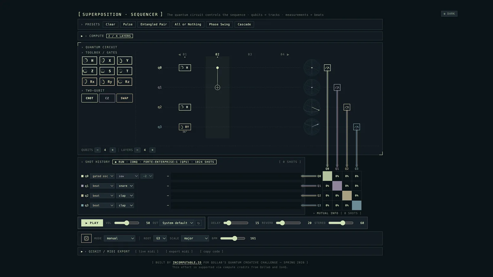Superposition SequencerFrancisco Estivallet · u/incomputable · Python + QiskitFrancisco Estivallet built a quantum music sequencer where every note comes from a circuit you design, turning a quantum computer into a playable instrument.

A coin gives you one distribution. A rotation gives you a dial, and ry is the dial. A dial is the first thing separating a superposition from a random number generator.

The angle the counts never show

A qubit's state has a second angle, and it does not appear in your results at all.

trigger_probability above takes θ and nothing else. The second angle is φ, the phase: the relative angle between the 0 and 1 halves of the state. The sequencer's other mapping takes φ and does something completely different with it:

​MAX_SWING = 0.35  # fraction of beat interval
​​
​def swing_offset(phi: float, max_swing: float = MAX_SWING) -> float:
​    """Map azimuthal angle φ in [0, 2π) to swing in [-max_swing, +max_swing]."""
1    normalized = (phi % (2 * math.pi)) / (2 * math.pi)
2    return (2 * normalized - 1) * max_swing
1φ is the phase: the relative angle between the 0 and 1 halves of the state.
2φ=0 plays maximally early, φ=π lands on the grid, φ approaching 2π plays maximally late.

Two circuits with the same θ and different φ draw from the same distribution. Run enough shots and the two tallies converge on each other; the differences that remain are shot noise, not φ. The sequencer still plays them differently, because it does not read φ off the shots. Instead it reads φ off a simulated state, and uses the shots only to decide which beats fire.

Phase is real, an rz gate sets it deliberately, and measuring straight away never reports it. Understanding Quantum Measurement makes the same point about the z gate from the other direction: a sign flip changes the state and changes no count.

This is also where the word weight has been doing quiet work. A weight is not only a size: it carries a sign, and phase is what sets that sign. Two probabilities can only ever add up, but two weights of opposite sign subtract.

So phase becomes visible when two routes to the same outcome meet and their weights either reinforce or cancel. That mechanism is what turns a flat superposition into an answer, and it is a subject of its own: Understanding Quantum Interference is the article about it.

Four superpositions, or one?

The sequencer's sampling module opens with a warning. The mistake it guards against is easy to make and hard to see:

​"""Correlated measurement sampling from the full statevector.
​​
​IMPORTANT (spec §16.2): for entangled qubits, sampling each qubit independently
​from its marginal destroys the correlations. Always sample bitstrings from the
​full statevector's probability distribution.
​"""
​​
​def sample_correlated(sv: Statevector, num_shots: int, rng=None) -> list[str]:
1    probs = sv.probabilities()
​    probs = probs / probs.sum()
​    n = sv.num_qubits
2    indices = rng.choice(len(probs), size=num_shots, p=probs)
​    return [format(int(i), f"0{n}b") for i in indices]
1One probability per outcome of the whole register. Four qubits means sixteen numbers here, not four.
2Each shot draws one outcome from that joint distribution. Whatever correlations the circuit built survive the draw.

Four qubits each sitting at fifty-fifty is not four coins. It is one distribution over sixteen outcomes, and only if the qubits are unentangled do those two descriptions agree. Add one cx and they part company: the per-qubit odds can look completely unchanged while the joint distribution has become something else entirely.

A marginal is the distribution for one qubit once you ignore the others. Sample each qubit from its own marginal and you get four independent coins every time, which is a valid distribution and the wrong one. The sequencer's README is blunt about what that costs musically: the entanglement presets become meaningless noise, where sampling the joint distribution keeps two entangled qubits firing together.

So superposition is a property of the register, not a property you can inspect qubit by qubit and reassemble. Understanding Quantum Entanglement is the article about what the difference buys you.

Twenty-four gates, sixteen million splits

Twenty-four Hadamards is the two-qubit circuit above, carried twenty-two doublings further.

Dr. Siti Fariya's Quantum Courier races classical and quantum solvers across logistics problems. Its repository carries a separate MaxCut benchmark, which is the piece that maps onto a circuit most directly.

MaxCut splits the nodes of a graph into two groups so that as many edges as possible run between the groups rather than inside them. The benchmark uses twenty-four nodes with three edges each, thirty-six edges in total. Splitting twenty-four nodes two ways gives 16,777,216 possible splits, which is the same number the ladder above arrived at, for the same reason.

A graph is not written in gates, so it gets rewritten twice before it becomes a circuit. First as a cost function: every edge contributes -x_u - x_v + 2·x_u·x_v, which is at its lowest when the two endpoints land on opposite sides. Then the substitution x = (1 - z)/2 turns those 0/1 variables into -1/+1 spins, which is exactly what measuring a qubit gives you.

Single-variable terms then become an rz on one qubit. Each edge's paired term becomes the cx, rz, cx sandwich. Every edge of the graph is literally a two-qubit gate in the circuit.

​def build_maxcut_qaoa(h: dict, J: dict, n: int, gamma: float, beta: float):
​    """Build the standard depth-1 QAOA circuit for MaxCut."""
​    from qiskit import QuantumCircuit
​    qc = QuantumCircuit(n, n)
​​
​    # Initial state: uniform superposition
1    qc.h(range(n))
​​
​    # Cost layer: exp(-i * gamma * H_cost)
​    for i, hi in h.items():
​        if abs(hi) > 1e-12:
​            qc.rz(2 * gamma * hi, i)
​    for (i, j), Jij in J.items():
​        if abs(Jij) > 1e-12:
​            qc.cx(i, j)
2            qc.rz(2 * gamma * Jij, j)
​            qc.cx(i, j)
​​
​    # Mixer layer: exp(-i * beta * H_mixer)
​    for i in range(n):
3        qc.rx(2 * beta, i)
​​
​    qc.measure(range(n), range(n))
​    return qc
1One Hadamard per node. With n=24 that is twenty-four gates, and the register now carries equal weight on all 16,777,216 possible splits.
2One interaction per edge. It shifts phase by an amount that depends on whether that edge ends up cut.
3The mixer moves weight between splits, so the circuit is not stuck with the distribution the cost layer handed it.

gamma and beta are two numbers, and the circuit above is only one evaluation of them. A classical optimiser sits outside it, rebuilding and rerunning the whole circuit at each step and adjusting the pair from what comes back. It starts at gamma = π/8 and beta = π/4, which the repo takes from the 2014 QAOA paper by Farhi, Goldstone and Gutmann. The 0.393 and 0.785 in Quantum Courier's Playground excerpt are those two constants rounded.

The committed benchmark ran five random graphs at 4,096 shots on a local simulator, and QAOA beat the classical baseline on all five, averaging about 43% more cut edges.

That baseline is a one-step local search where each node decides using only its immediate neighbours and never sees the whole graph. The repo picks it deliberately and cites Carlson et al. 2023 for the choice. At depth 1 the quantum circuit also reaches only one edge away from each node, so it argues that a solver with a global view would not be like-for-like.

Twenty-four gates bought weight on 16,777,216 outcomes. The 4,096 shots read back 0.024% of them.

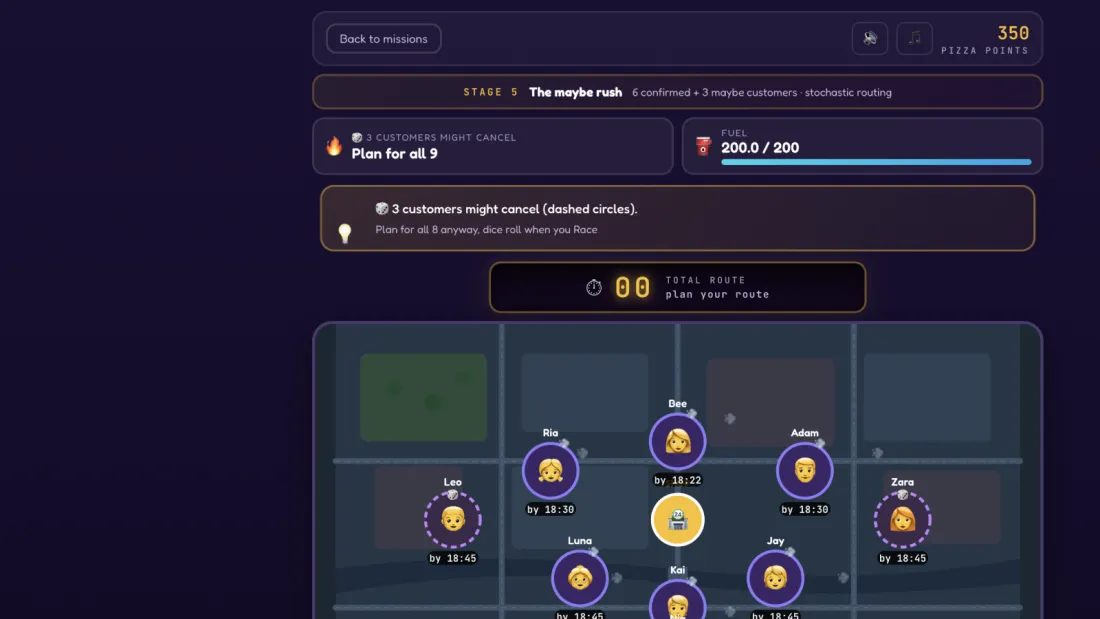Quantum CourierDr. Siti Fariya · u/Sitifar · Python + QiskitDr. Siti Fariya built a browser game that races classical and quantum solvers across five real logistics problems, and shows honestly which one wins, and why.

Why the rest of that circuit exists

If a flat superposition were an answer, build_maxcut_qaoa would stop after its first line. It does not, and the reason is the 0.024%.

An even mix over sixteen million splits, sampled 4,096 times, gives you 4,096 arbitrary splits. That is a slow, expensive way to guess. Everything after qc.h(range(n)) exists to move weight off the bad splits and onto the good ones, so that when you do take those 4,096 samples they land somewhere worth looking.

The two layers split the work. One cx, rz, cx sandwich per edge shifts phase by an amount that depends on whether that edge is cut. Splits that cut more edges end up with a different phase from splits that cut fewer. The mixer then converts those phase differences into differences in weight. Both layers are parameterised by gamma and beta, and tuning those two numbers is what the surrounding optimiser spends its time on.

Phase differences turning into weight differences is interference. Why the cancellation lands where it does is a subject of its own, and Understanding Quantum Interference is the article about that.

The benchmark result committed to Quantum Courier's repository was produced on a local simulator, over five random graphs, against a classical one-step search. There is an IonQ path in the script too. Which of those a figure came from is worth checking before repeating it.

The simulator has the amplitudes, the hardware never will

The sequencer's interface shows you a Bloch sphere per qubit and the amplitudes of the full state, updating as you add gates. Alongside that, it plays audio driven by measurements. Those are two different code paths, and only one of them could ever run on a quantum computer.

​def state_at_step(spec: CircuitSpec, step: int) -> StepState:
​    qc = build_subcircuit(spec, up_to_step=step)
​    bloch = get_bloch_vectors(qc)
1    sv = Statevector.from_instruction(qc)
2    return StepState(step=step, bloch_vectors=bloch, statevector=_amplitudes(sv))
1Computes the state directly. No shots, no sampling: the actual complex amplitude of every basis state.
2_amplitudes hands the browser a real and an imaginary part per outcome, which is what draws the spheres and the bars.

Statevector.from_instruction is a simulator doing linear algebra. It can tell you the weight and the phase on every one of the register's outcomes, which is precisely the information a measurement destroys. That is why the sequencer's visuals are exact and its audio is sampled.

Run the same circuit on hardware and state_at_step has no counterpart. There is no call that returns the state, because there is no way to look at a quantum state without ending it. You get a tally.

Keep a simulator in the loop while you are still learning a circuit. Once the register grows, it stops being an option.

What a real machine does to a superposition

There is a second number the sequencer reads off each qubit, and it is the one that connects all of this to hardware.

​for q in range(n):
​    others = [i for i in range(n) if i != q]
1    rho = partial_trace(sv, others).data
​    r_x, r_y, r_z = _bloch_from_density(rho)
​​
2    r = float(np.sqrt(r_x * r_x + r_y * r_y + r_z * r_z))
1Throws away every other qubit and keeps what is left of this one on its own.
2The length of that vector. r=1 means the qubit has a state of its own; r below 1 means the description is incomplete.

The sequencer maps r to timbre, and the README is explicit that this is a decision not to hide something. Entanglement makes an individual qubit's state mixed, and the instrument treats that as real physics to be heard rather than a value to normalise away. Its velocity mapping turns a shorter vector into a quieter note.

On real hardware r shrinks for a second reason. Superpositions are not stable. It decays into the environment, every gate takes time, and a circuit deep enough to be interesting is a circuit spending that time. What arrives as your counts is a mix of the distribution you designed and one you did not.

Shivani Mayekar's QuantumCanvas handles that with one line:

​counts = job.get_counts()
1counts = {b: c for b, c in counts.items() if c > shots * low_prob}
1Drops outcomes that turned up too rarely to be signal. With low_prob=0.05, anything under 5% of the shots goes.

For a Bell state, a pair of entangled qubits that should only ever produce 00 and 11, that filter removes the 01 and 10 counts that hardware puts there anyway. It is a blunt instrument and it works because you knew what the answer was supposed to look like. On a circuit whose answer you do not already know, the same filter would happily delete a real result.

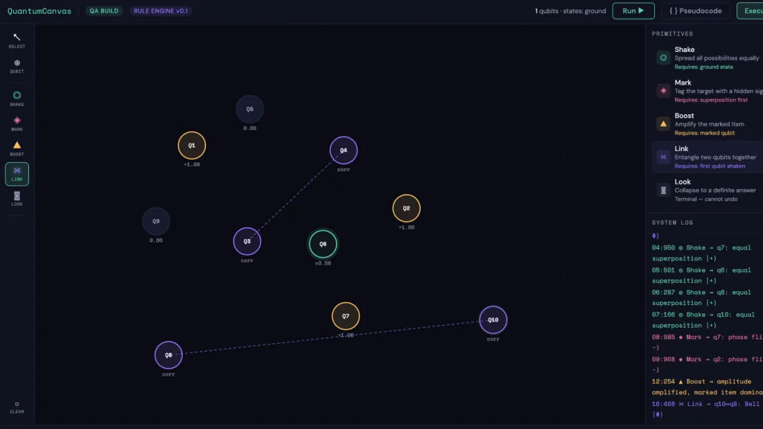QuantumCanvasShivani Mayekar · u/ShivaniMayekar · Python + QiskitShivani Mayekar built a visual sandbox where you drag and drop quantum operations to compose new algorithms, then run them on real hardware.

Choosing where your code runs covers the backends available on Qollab. Why your results look wrong covers what to check when a circuit ran cleanly and still gave you something unexpected.

Start with one qubit

Superposition is a set of weights you compose before you measure. Four consequences of that keep mattering.

An even spread of weights is cheap to create and expensive to read, so the interesting work is never in setting that up. Part of the state never reaches your counts, which is why phase can decide an algorithm and show up nowhere in a tally. Weights belong to the whole register, so a superposition cannot be inspected one qubit at a time and reassembled. And on hardware they decay while the circuit runs, so depth costs you accuracy.

Fork the Superposition Sequencer first. It is the fastest way to see the first of those. You change an angle and hear the rhythm change, and the number you dialled and the pattern you hear are connected by three lines of Python and nothing else.