Quantum Chemistry and VQE
VQE finds a molecule's ground-state energy by preparing a trial state on qubits and measuring it, one tally per measurement basis. On hydrogen the 20 mHa of correlation energy only shows once the X basis is read as well. Code to run and fork.

About the author
Quantum chemistry on a quantum computer means finding a molecule's ground-state energy, the energy its electrons settle into. You prepare a trial version of the electrons' ground state on qubits and measure the energy.
VQE, the variational quantum eigensolver, is the standard way to find a ground-state energy on today's machines. A circuit with a few knobs prepares the trial state, a tally of repeated measurements gives its energy, and a classical optimizer changes the knobs until the energy stops falling.
The smallest version has one qubit, one rotation and a measurement, and its energy is the average of the readings. Hydrogen runs the same loop on two qubits and lithium hydride on ten. The Hamiltonian, the list of weighted measurements that defines each energy, comes from PySCF and qiskit-nature, and two of the projects describe taking the same loop to IonQ hardware.
What is quantum chemistry on a quantum computer?
A molecule's ground-state energy is the energy of its electrons' lowest-energy arrangement. That energy, taken at each position of the nuclei, decides the bond length, the energy a reaction releases, and whether the molecule holds together. Working the ground-state energy out exactly gets exponentially expensive on a classical computer, because the electron state has one weight for every way of filling the available electron slots.
A quantum computer can hold the electron state once the electrons are encoded as qubits, one qubit per orbital slot in the direct encoding, Jordan-Wigner. VQE, the variational quantum eigensolver, prepares a trial state with a circuit that has a few knobs and measures its energy one measurement setting, or basis, at a time.
A classical optimizer turns the knobs until the energy stops falling. The estimate is the lowest energy the optimizer reaches. No trial state has an energy below the true ground-state energy (the variational principle), so before shot noise the estimate can only be too high. The estimate equals the true energy only if the circuit can reach the ground state and the optimizer finds it. The measured number then scatters to either side of that, because a finite tally is noisy.
Hydrogen and lithium hydride are small enough to solve exactly on a laptop. The Hamiltonian's list of terms grows, before any grouping, roughly as the fourth power of the number of orbitals, and at a few dozen orbitals the exact method exceeds any computer. Whether VQE reaches that size on noisy hardware is not settled.
Hydrogen has two protons, two electrons, and a ground-state energy of −1.137 hartree at a bond length of 0.735 ångström in the smallest model chemists use. Every project and listing computes hydrogen's ground-state energy, or lithium hydride's, or a toy Hamiltonian's.
A hartree is the unit of energy in electronic-structure calculations. The energy differences that decide a reaction are hundredths to tenths of a hartree, and ranking two reactions needs them to about a thousandth of a hartree, so the working unit is the millihartree. Chemists call 1.6 millihartree, about 1 kcal/mol, chemical accuracy: an energy within it is close enough for reaction energies to be trusted.
The bond-length curve
The bond-length curve is hydrogen's energy recomputed at each distance between the two protons. The position of its lowest point is the bond length, and its depth, against two separate atoms far apart, is the bond energy. A large part of chemistry on a computer is computing curves like hydrogen's for larger molecules.
Three terms recur:
- Hartree-Fock: the best energy you get by treating each electron as moving in the average field of the others. Hartree-Fock puts the electrons in one definite set of orbitals: one string of occupied and empty slots. An orbital is a region an electron can occupy around the nuclei, with room for two electrons.
- Exact: the lowest energy the model allows, found by writing the Hamiltonian out as a matrix and solving for its lowest eigenvalue, diagonalising it, when the model is small enough for that.
- Correlation energy: the gap between the Hartree-Fock and exact energies: the part of the energy that one definite set of orbitals cannot describe.
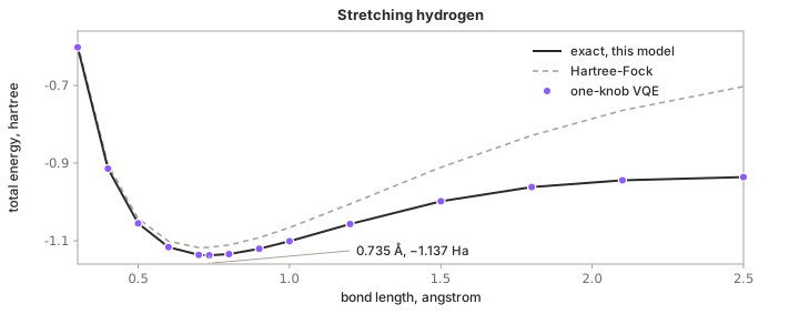
At the bond length the correlation energy is 20 mHa, almost thirteen times chemical accuracy. At 2.5 Å the correlation energy is 233 mHa. The classical methods that scale to big molecules build on one string of orbitals, and their error grows as a bond breaks.
Qollab's quantum-chemistry-showcase-t-2 example, the bond-length slider, draws the dissociation curve live: drag the bond length and a four-parameter VQE re-solves the energy in your browser at every position.
Where quantum chemistry came from
Six milestones, from the first quantum-mechanical account of a chemical bond in 1927 to the hardware experiments of 2025:
In 1928 Jordan and Wigner wrote down how to turn electrons, which never share a state (the exclusion principle), into two-level systems, which have no such rule. Hartree in 1928 and Fock in 1930 gave the average-field method that still supplies the starting string for the hydrogen listing and for qOrbital's UCCSD.
Hydrogen has been run on superconducting qubits since 2016, and Google's 2020 Hartree-Fock experiment used a chain of twelve qubits. The molecules stayed small because the term count and the noise both grow with the orbitals.
What one energy evaluation does
A Hamiltonian, on a quantum computer, is a list of measurements with weights. Each entry names a measurement (the Z reading of a qubit, the product of two readings, or a reading taken after a rotation) and gives it a coefficient. An exact solver diagonalises that same list, written out as a matrix.
A basis is which measurement is taken. A plain measure on a qubit is the Z reading. The same measure after an h rotation is the X reading, and a third basis, Y, needs one more gate in front. Hydrogen needs Z and X.
The molecule's energy is the weighted sum of the entries' readings, each averaged over many shots.
One shot gives 0 or 1, scored as +1 or −1. Take a thousand shots of the same trial circuit, average the scores, and the average is the number the coefficient multiplies. An energy evaluation is a few tallies, one per measurement basis, each multiplied by its coefficient and added together.
On one qubit with two terms, Z and X, one evaluation is two tallies. Prepare the trial state and read it in Z: that tally gives the Z term its average.
Prepare the trial state again, rotate with an h, and read the state in Z again: that tally is the X reading, because the rotation turns X into Z. Multiply each tally by its coefficient and add the two; the optimizer then changes the knob.
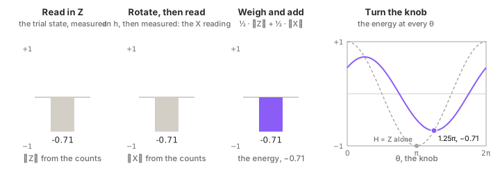
The optimizer works from the fourth panel, the energy at every setting of the knob: the optimizer evaluates the energy at the current setting and at a second setting, and keeps whichever setting gave the lower energy. With Z alone the minimum is at π: flip the qubit and read −1.
Add the X term and the best state is a superposition, the minimum moves to 1.25π and −0.707, and reading in one basis alone would never find it.
The smallest circuit you can make
A trial state with one knob is one rotation. Read the trial state in Z and average the readings, and the average is the energy for a Hamiltonian that is Z alone. The run button under each listing opens Qollab's VQE example: fork it, paste the listing over the example's code, and run the listing.
# 'backend' is pre-created for you in the Qollab Playground.
from math import pi
from qiskit import QuantumCircuit
1theta = pi
SHOTS = 1000
qc = QuantumCircuit(1, 1)
2qc.ry(theta, 0)
qc.measure(0, 0)
counts = backend.run(qc, shots=SHOTS).result().get_counts()
3z = (counts.get("0", 0) - counts.get("1", 0)) / SHOTS
4print(z)
- 1The knob. A circuit with a knob in it is called an ansatz, and one rotation is the smallest ansatz.
- 2The trial state. At
theta = 0 the qubit stays at 0; at pi it is flipped to 1; in between it is a superposition of the two. - 3The average Z reading: +1 for every
0, −1 for every 1. For a Hamiltonian that is Z alone, the average Z reading is the energy. - 4−1.0 at
theta = pi, +1.0 at 0, about 0 at pi / 2. The energy is cos(theta), and the lowest it gets is −1, at pi.
Now give the Hamiltonian a second term, ½ Z + ½ X. The X reading needs the rotation, so the evaluation is two circuits:
# 'backend' is pre-created for you in the Qollab Playground.
from math import pi
from qiskit import QuantumCircuit
1theta = 1.25 * pi
SHOTS = 1000
def average(basis):
qc = QuantumCircuit(1, 1)
2 qc.ry(theta, 0)
if basis == "X":
3 qc.h(0)
qc.measure(0, 0)
counts = backend.run(qc, shots=SHOTS).result().get_counts()
return (counts.get("0", 0) - counts.get("1", 0)) / SHOTS
4energy = 0.5 * average("Z") + 0.5 * average("X")
5print(energy)
- 1The knob, set to the angle that gives this Hamiltonian its lowest energy.
- 2The same trial state as
vqe_one_qubit.py. - 3Rotate before reading, so that a Z measurement reports X. The two tallies differ only in this line.
- 4Each tally is multiplied by its coefficient and the two products are added: the weighted sum from the four panels, in one line.
- 5About −0.71. Set
theta to pi and it reads −0.5: the Z reading is −1, its lowest, and the X reading is zero. Each reading reaches −1 at some angle, but no single angle gives both readings −1.
Between π and 1.25π the Z reading rises from −1 to −0.71 and the X reading falls from 0 to −0.71, and the best angle has the lowest weighted sum. Hydrogen's knob moves its two readings against each other in the same way.
The gates in these circuits
Four gates and one instruction cover the three teaching listings. The project excerpts add a few more, named where they appear.
A rotation with a knob. On a qubit at 0 it leaves a superposition of 0 and 1 whose balance the angle sets, and at pi it flips the qubit. The trial states in the teaching listings are made of ry gates, and the optimizer changes their angles.
Flips a qubit, 0 to 1. Hydrogen's circuit opens with one, to write the Hartree-Fock string before the rotation is applied.
CNOT
Flips the second qubit when the first is 1. When the first qubit is in superposition, this ties the two into one shared state, and in hydrogen's circuit it moves weight from one string of orbitals to another.
Hadamard
On a qubit at 0 it gives equal weight to 0 and 1. Placed just before a measurement, h turns an X reading into a Z reading; a machine only ever reads Z, so an X term is read this way.
Reads a qubit into an ordinary bit and forces it to a definite 0 or 1. One run gives one string, so every energy read from a real device is an average over thousands of runs, and the shot count is a cost of its own on a machine.
Hydrogen on two qubits
Hydrogen in the smallest sensible model, one orbital per atom, STO-3G in the code, has four slots for electrons, two per orbital, and two electrons to put in them. The direct encoding, Jordan-Wigner, uses one qubit per slot: four qubits.
The number of electrons of each spin is fixed, one up and one down, so two of the four qubits only ever repeat what the other two already say. The parity encoding stores in each qubit whether an odd number of the slots up to that one are filled, instead of each slot on its own. With the electron counts fixed, two of the parity qubits never change; the encoding drops them, and hydrogen becomes two qubits and five terms at every bond length.
The table is the electronic Hamiltonian, energies in hartree, as the two chemistry packages of a later section, PySCF and qiskit-nature, print it. Qollab's quantum-chemistry-showcase-the example, the dissociation curve with VQE, carries one such row for each of fourteen bond lengths, and this is its 0.735 Å row. A term's two letters name qubit 1 then qubit 0, and I means that qubit is left out of the reading:
| term | coefficient | read in |
|---|---|---|
| II | −1.052373 | no circuit: a constant |
| IZ | +0.397937 | Z |
| ZI | −0.397937 | Z |
| ZZ | −0.011280 | Z |
| XX | +0.180931 | X, after an h on both qubits |
The table is the electrons' energy only. The nuclear repulsion, the two protons pushing each other apart, is a separate constant, +0.719969 Ha, added at the end to make a total. The Hartree-Fock string in this encoding is 01, and its total energy is −1.116999 Ha. The exact ground state is −1.137306 Ha, 20 mHa lower.
The trial state that reaches the ground state has one knob. Prepare 01, rotate qubit 1, and apply a CNOT from qubit 1 to qubit 0. The result is a mix of 01 and 10, the string with both electrons moved up to the higher orbital, and the knob sets the mix.
# 'backend' is pre-created for you in the Qollab Playground.
from qiskit import QuantumCircuit
1theta = -0.2235
SHOTS = 10000
2H2 = {
"II": -1.052373, "IZ": 0.397937, "ZI": -0.397937,
"ZZ": -0.011280, "XX": 0.180931,
}
NUCLEAR = 0.719969
def trial():
qc = QuantumCircuit(2, 2)
3 qc.x(0)
qc.ry(theta, 1)
4 qc.cx(1, 0)
return qc
def tally(basis):
qc = trial()
if basis == "X":
5 qc.h([0, 1])
qc.measure([0, 1], [0, 1])
return backend.run(qc, shots=SHOTS).result().get_counts()
def average(counts, term):
total = 0
6 for string, n in counts.items():
sign = 1
for bit, pauli in zip(string, term):
if pauli != "I" and bit == "1":
sign = -sign
total += sign * n
return total / SHOTS
BASES = ("Z", "X")
parts = {}
if "Z" in BASES:
z_counts = tally("Z")
7 parts["Z"] = sum(H2[t] * average(z_counts, t) for t in ("IZ", "ZI", "ZZ"))
if "X" in BASES:
x_counts = tally("X")
8 parts["X"] = H2["XX"] * average(x_counts, "XX")
print(parts)
if len(parts) == 2:
9 print(H2["II"] + parts["Z"] + parts["X"] + NUCLEAR)
- 1The one knob. 0 is the Hartree-Fock string; −0.2235 is the ground state, derived exactly for this Hamiltonian.
- 2Hydrogen at 0.735 Å on two qubits, the table above. A constant, three terms read in Z, one read in X.
- 3
x flips qubit 0 from 0 to 1, which writes the Hartree-Fock string 01: both electrons in the lower orbital, in the parity encoding. - 4The knob and the CNOT together move weight from
01 to 10. At 0 nothing moves and the state is Hartree-Fock. - 5Rotate both qubits before reading, so that a Z readout reports X. The same trick as the one-qubit listing, on two qubits at once.
- 6A string reads
q1 q0, the same order as a term's letters. Every 1 under a Z or an X flips the sign of that shot. - 7The three Z-basis terms, all read from the one Z tally.
- 8The X-basis term, read from the second tally. Set
BASES to ("Z",) and the printed Z part rises from −0.785 to −0.765; add the constants and the ground state reads 19.8 mHa above Hartree-Fock, because the X term that lowers it is missing. - 9About −1.137 Ha, within the 2.5 mHa that 10,000 shots scatter by. Set
theta to 0 and the line prints about −1.117, the Hartree-Fock energy. Set theta to +0.2235 and the line prints about −1.057: the sign of the knob decides whether the X term lowers the energy or raises it.
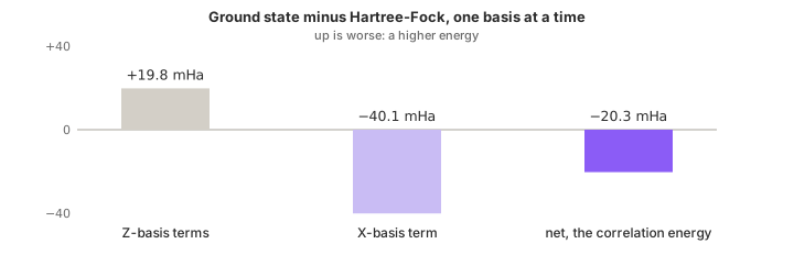
Moving the knob raises the Z-basis terms and lowers the X-basis term; the figure plots the two parts against the angle. As theta moves from 0 towards −0.22 the Z-basis terms rise: with the II constant and the nuclear constant added, their part goes from −1.117 to −1.097 Ha, 19.8 mHa. The listing's parts["Z"] prints the same rise without the constants, −0.785 to −0.765. The X-basis term, zero at Hartree-Fock, falls to −0.040 Ha. The total falls by the net of the two, 20.3 mHa: the correlation energy.
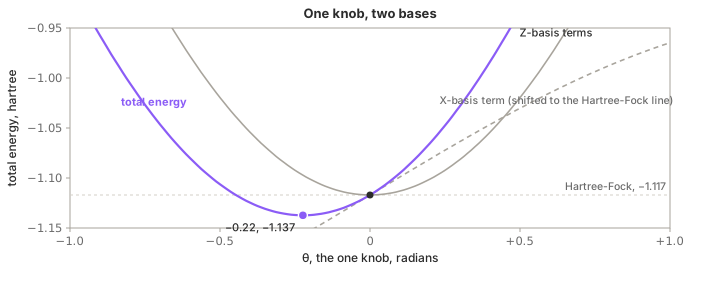
Read the ground state in Z alone, with BASES set to ("Z",) and the constants added to the printed part, and the energy reads −1.097 Ha, 19.8 mHa above Hartree-Fock: the rise in the Z-basis terms. The X tally supplies the 40.1 mHa drop.
The ground state at −0.2235 and the wrong-sign state at +0.2235 give the same Z tally, 98.8% 01 and 1.2% 10, and that tally does not show which of the two has the lower energy.
A second basis is the only difference in what the machine measures between VQE on a molecule and QAOA: a QAOA cost has only Z terms, it is diagonal, so one Z tally gives every term its average; a molecule's Hamiltonian is not diagonal, so a second basis is always needed.
The optimizer that turns the knob is the same classical loop in both cases.
Where the Hamiltonian comes from
Hydrogen's five coefficients come from a classical calculation. PySCF, a chemistry package, computes the integrals between the orbitals: how much energy each electron has in each orbital and how strongly pairs of electrons repel. The integrals are the Hamiltonian written for electrons, which hop between orbitals and cannot share one.
A qubit can store an occupation directly, but not the sign that flips when two electrons swap places, so the second step is an encoding that keeps that sign. Qollab's showcase-fermionic-op example maps the simplest electron term, a hop between two orbitals, onto Pauli strings, letter labels like the XX in hydrogen's table, with the Jordan-Wigner transformation:
1op = FermionicOp({"+_0 -_1": 1.0, "+_1 -_0": 1.0}, num_spin_orbitals=2)
print("Fermionic operator (second quantization):")
print(op)
# The Jordan-Wigner transform: orbital occupation <-> qubit basis state,
# with Z-strings preserving the fermionic sign structure
2qubit_op = JordanWignerMapper().map(op)
print(f"\nMapped onto {qubit_op.num_qubits} qubits as Pauli strings:")
print(qubit_op)
- 1Written for electrons: create an electron in orbital 0 and remove one from orbital 1, plus the reverse, a hop between the two orbitals.
- 2The same hop written for qubits. The mapped operator prints as a
SparsePauliOp with the labels YY and XX at 0.5 each: two terms a circuit can measure, neither of them in the Z basis; a Y reading is an X reading with one more gate, sdg, in front of the h. Every X and Y term in these Hamiltonians comes from a hop like this one.
Hops between orbitals become XX and YY terms, and the number of electrons in an orbital becomes a constant plus a Z term. Hydrogen's XX is its two electrons hopping together from the lower orbital to the upper one, and the Z terms are the energies of occupying each orbital. In hydrogen's four-qubit form that double hop is four terms mixing X and Y across all four qubits; the two-qubit form folds them into the one XX row of the table.
Qollab's showcase-h2-ground-state example runs the full pipeline from first principles, in the browser, on a WebAssembly build of PySCF. The example ends with an exact solver rather than VQE, because at four qubits the matrix is small enough to diagonalise:
from qiskit_algorithms import NumPyMinimumEigensolver
from qiskit_nature.second_q.algorithms import GroundStateEigensolver
from qiskit_nature.second_q.drivers import PySCFDriver
from qiskit_nature.second_q.mappers import JordanWignerMapper
1solver = GroundStateEigensolver(JordanWignerMapper(), NumPyMinimumEigensolver())
# Scan the H-H bond length around the known equilibrium (~0.735 angstrom)
print("bond length (A) total energy (Hartree)")
best = None
for dist in (0.5, 0.735, 1.0, 1.5):
2 problem = PySCFDriver(atom=f"H 0 0 0; H 0 0 {dist}").run()
energy = float(solver.solve(problem).total_energies[0].real)
if best is None or energy < best[1]:
best = (dist, energy)
3 print(f" {dist:5.3f} {energy:+.6f}")
print(f"\nMinimum of the scan at {best[0]} A with {best[1]:+.6f} Ha")
print("(textbook equilibrium: about -1.137 Ha at 0.735 A)")
- 1The encoding and the solver.
NumPyMinimumEigensolver diagonalises the matrix; the showcase-vqe-ground-state listing puts VQE in its place. - 2PySCF runs Hartree-Fock and builds the integrals for this geometry. Four qubits under Jordan-Wigner, one per slot.
- 3−1.055160, −1.137306, −1.101150 and −0.998149 Ha, the curve's exact values at these four points. The two-qubit encoding, one coefficient row per bond length in the dissociation example, gives the same four numbers.
Both encodings give the same curve on different qubit counts. Bigger molecules need more qubits either way, and the term count grows faster than the qubit count.
Qiskit Nature showcase: the ground-state energy of the hydrogen moleculeA complete quantum chemistry calculation from first principles, in the browser: PySCF computes the H₂ molecular integrals, qiskit-nature maps the electrons onto qubits via Jordan-Wigner, and an eigensolver finds the ground-state energy. The example scans the bond length and locates the equilibrium geometry.VQE from the Qiskit library
Qiskit's VQE class does in a few lines what the hydrogen listing did by hand: an estimator produces the energy of the trial state, and the class passes that energy to the optimizer. Qollab's showcase-vqe-ground-state example runs VQE on a two-qubit toy Hamiltonian:
# A toy 2-qubit Hamiltonian written as a sum of Pauli terms
1hamiltonian = SparsePauliOp.from_list([("II", -1.0), ("ZZ", 0.5), ("XX", 0.5)])
# The ansatz: layers of single-qubit RY rotations entangled with CZ gates
2ansatz = n_local(2, "ry", "cz", reps=1)
ansatz.draw("mpl", filename="ansatz.svg")
# Record how the energy estimate improves while the optimizer iterates
history = []
def track(eval_count, params, value, meta):
3 history.append(value)
4vqe = VQE(StatevectorEstimator(), ansatz, COBYLA(maxiter=50), callback=track)
result = vqe.compute_minimum_eigenvalue(hamiltonian)
# Cross-check against exact diagonalization (feasible for tiny systems only)
exact = NumPyMinimumEigensolver().compute_minimum_eigenvalue(hamiltonian)
print(f"VQE estimate: {float(np.real(result.eigenvalue)):+.6f}")
5print(f"Exact answer: {float(np.real(exact.eigenvalue)):+.6f}")
- 1The list of weighted measurements, in Qiskit's form. A
ZZ term and an XX term: two bases again. - 2A trial circuit with several knobs, built from a library:
ry knobs with cz gates between them, a two-qubit gate that flips a sign when both qubits are 1. The hydrogen listing's x, ry, cx was one written by hand. - 3Every value the optimizer receives is the energy of one trial state. With
StatevectorEstimator the value is exact; on a device it would be the weighted sum of tallies the hydrogen listing assembled by hand. - 4The estimator supplies the energy, the ansatz is the trial state, and COBYLA changes the knobs.
StatevectorEstimator computes the exact average, the number a tally would settle on with unlimited shots, and takes no shots; a backend-based estimator builds one measurement circuit per basis instead. - 5An exact answer to compare against, available only while the molecule is small enough to diagonalise.
Run the example and the estimate usually ends close to the exact answer, −2, within fifty evaluations. The history list differs from run to run because the optimizer starts at a random point, and some starts have not reached −2 after the fiftieth evaluation; the number printed is then the energy at the optimizer's last point, above the minimum.
The optimization article covers how the optimizer moves from one point to the next; VQE uses the same loop, on an energy with a known floor, the ground state.
Qiskit Algorithms showcase: ground-state energy with VQEThe Variational Quantum Eigensolver (VQE) is the flagship near-term quantum algorithm: a small parameterized circuit is trained by a classical optimizer to find the lowest eigenvalue of a Hamiltonian. This example minimizes a two-qubit Hamiltonian, tracks the optimizer convergence, and checks the result against the exact answer.The quantum-chemistry-showcase-the example, the dissociation curve with VQE, runs the loop at fourteen bond lengths, with a two-knob-per-layer ansatz and an optimizer written in plain Python. The example's VQE comes within 0.02 mHa of exact at every point.
Two things to try when you fork the example: in its file, set REPS = 1 and see whether one layer is enough, and add shot noise to its energy() function, its own docstring's suggestion, to see the curve scatter.
Two kinds of ansatz
The trial circuit limits which states VQE can prepare, and two published Qollab projects take opposite approaches to it.
qOrbital's ansatz, UCCSD, starts from the Hartree-Fock string and adds the two kinds of electron move that account for most of the correlation energy, single and double hops. Aryan Bawa and Arnav Singh's Playground file builds the full pipeline from the molecule's name:
# UCCSD ansatz starting from the Hartree-Fock reference state.
1initial_state = HartreeFock(problem.num_spatial_orbitals, problem.num_particles, mapper)
ansatz = UCCSD(
problem.num_spatial_orbitals, problem.num_particles, mapper, initial_state=initial_state
2)
optimizer = {"SLSQP": SLSQP, "COBYLA": COBYLA}[OPTIMIZER](maxiter=MAX_ITERATIONS)
# The callback fires once per optimizer step -- print the electronic energy
# as it descends toward the minimum.
def show(eval_count, parameters, mean, metadata):
3 print(f" iter {eval_count:>3} E_elec = {mean:+.6f} Ha")
vqe = VQE(
estimator=StatevectorEstimator(),
ansatz=ansatz,
optimizer=optimizer,
callback=show,
initial_point=np.zeros(ansatz.num_parameters),
)
result = vqe.compute_minimum_eigenvalue(qubit_op)
- 1The starting string, built from the electron count and the encoding.
- 2The chemistry-inspired ansatz: one knob per electron move that chemistry allows. In this four-qubit encoding hydrogen gets three knobs, where the two-qubit circuit above needed one; lithium hydride gets ninety-two.
- 3The first line it prints is the Hartree-Fock energy, because the knobs start at zero, and with every knob at zero the circuit is the starting string. Every drop from that first value recovers part of the correlation energy.
Run the file on hydrogen with its default OPTIMIZER, SLSQP, and the first four evaluations all print −1.836968 Ha, the electronic Hartree-Fock energy: the optimizer probes each knob by a step too small to move the sixth decimal. The fifth evaluation is a step in the wrong direction, and the tenth prints −1.857275, the exact electronic energy. COBYLA reaches the same value by a longer route. Adding the nuclear constant to −1.836968 and −1.857275 gives −1.117 and −1.137 Ha, hydrogen's Hartree-Fock and exact totals.
Change MOLECULE to "LiH" and the same file builds lithium hydride, switching to the parity encoding with the two-qubit reduction for this molecule: ten qubits, a Hamiltonian of 631 terms, ninety-two knobs, and 1,035 evaluations to reach a total of −7.882 Ha. The lithium hydride run took almost an hour and a half on a laptop, outside the browser.
The project describes what it does with the state it finds: it reconstructs the electron density and draws the orbital as a cloud. The README also describes a bundled gallery of runs on IonQ hardware, overlaid so that the run-to-run noise shows as a cloud of trajectories instead of an error bar.
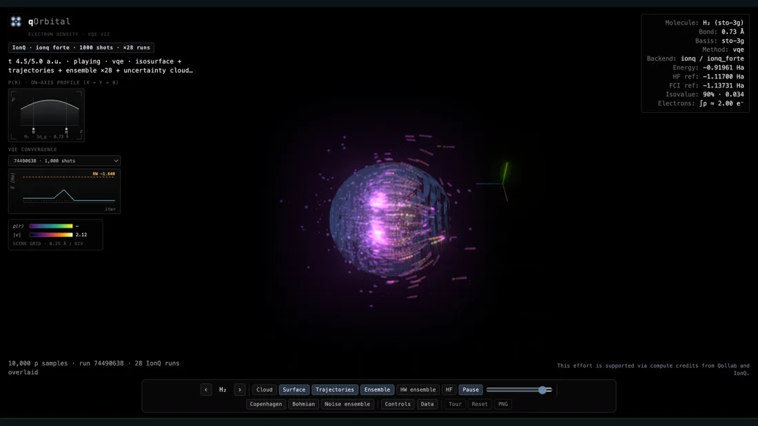 qOrbitalInteractive quantum chemistry orbital visualizer — compute molecular ground states with VQE on real quantum hardware and explore 3D electron density isosurfaces in the browser.
Quantum Advantage Lab's ansatz is written in the standard gates that map most directly onto a trapped-ion machine: rotations on every qubit, then an rxx interaction on every pair. Hossein Sadeghi's project races VQE against a classical solver on hydrogen and on a reduced four-qubit model of lithium hydride. Its README says rxx was chosen because it maps onto the Mølmer-Sørensen interaction; on IonQ's Aria systems one rxx is one native MS gate, and on Forte, the hardware behind Qollab's QPU backends, it compiles to one ZZ gate.
The two vqe.py excerpts below come from the project's GitHub repository; its Qollab page carries a different piece of the Lab, a Hamiltonian-simulation demo.
qc = QuantumCircuit(n_qubits, name="VQE_Ansatz")
idx = 0
for layer in range(depth):
# Single-qubit rotations
for q in range(n_qubits):
1 qc.ry(params[idx], q)
idx += 1
qc.rz(params[idx], q)
idx += 1
# All-to-all entangling: RXX between all pairs (native on IonQ via MS gate)
for i in range(n_qubits):
for j in range(i + 1, n_qubits):
2 qc.rxx(np.pi / 4, i, j)
qc.barrier()
# Final rotation layer
for q in range(n_qubits):
qc.ry(params[idx], q)
idx += 1
qc.rz(params[idx], q)
idx += 1
return qc
- 1Two knobs per qubit per layer,
ry then rz, a rotation the Z counts alone cannot see. The gates encode no chemistry. The layout, rotations on every qubit and one interaction per pair, matches the machine. - 2One
rxx on every pair of qubits, at a fixed angle. On a trapped-ion machine every qubit can interact with every other directly, so no routing gates are needed; on a chip with nearest-neighbour wiring this layer would need extra swap gates.
An ansatz built this way is called hardware-efficient. A hardware-efficient ansatz is short and cheap to run, and the Lab's run_vqe starts its knobs at seeded random values rather than at the Hartree-Fock string. The project's README says the race illustrates the structure of the optimization landscape, the energy at every knob setting, including the local minima that make VQE hard at scale.
A chemistry-inspired ansatz starts near the ground state and stays among states with the right electron count, and its circuit is deeper, which gives noise more gates to act on.
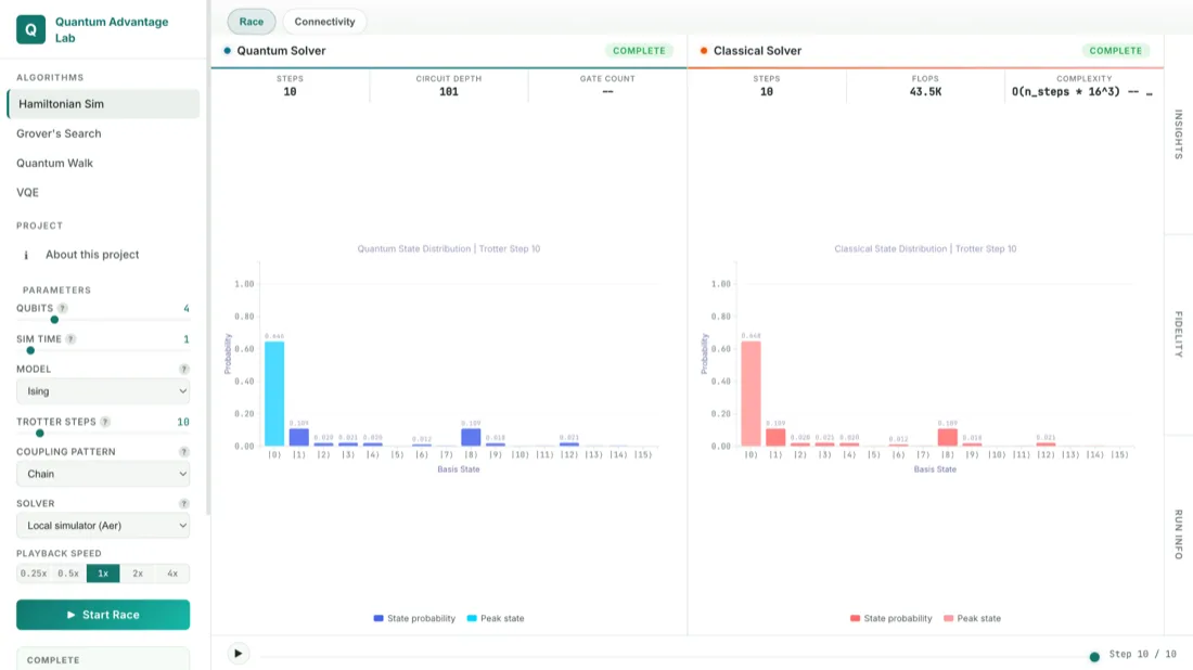 Quantum Advantage LabQuantum Advantage Lab is a real-time interactive platform that races four foundational quantum algorithms against their classical counterparts, making quantum speedups tangible by streaming each solver's progress side-by-side as the computation unfolds.
Measuring an energy on real hardware
Sending the converged circuit to a machine shows what the machine's own gate noise does to the trial state's energy, with no model in between.
Every listing that takes shots reads its X term with a second circuit, and the exact estimators skip the measuring altogether. On a machine the X term is a second circuit and a second job, hydrogen included. Terms that can share a basis share a tally, as hydrogen's three Z terms did, and Qiskit's backend estimators group terms that way before anything else.
The Lab's hardware path runs one job per term with no grouping, so it is the easiest form to read. Inside a loop over the Hamiltonian's terms, the code rotates the qubits each term needs into the Z basis: h for an X, sdg then h for a Y. Then the code measures and turns the tally into a signed average:
# Build measurement basis rotation
cr = meas_circuit
cb = QuantumCircuit(n_qubits, n_qubits)
for i, p in enumerate(reversed(pauli_label)):
if p == "X":
1 cb.h(i)
elif p == "Y":
cb.sdg(i)
cb.h(i)
cb.measure(range(n_qubits), range(n_qubits))
full = bound_circuit.compose(cb)
transpiled = transpile(full, backend=backend)
result = run_job_and_get_result(
backend,
transpiled,
shots=shots,
run_kwargs=run_kwargs or {},
execution=execution,
2 )
counts = result.get_counts()
# Expectation from counts
total_shots = sum(counts.values())
exp_val = 0.0
for bitstring, count in counts.items():
# Parity of measured qubits where Pauli is not I
parity = 0
for i, p in enumerate(reversed(pauli_label)):
if p != "I":
parity += int(bitstring[n_qubits - 1 - i])
3 sign = (-1) ** (parity % 2)
exp_val += sign * count / total_shots
energy += float(np.real(coeff)) * exp_val
- 1The rotation the hydrogen listing used, chosen per qubit from the term's letters. A Y needs one more gate.
- 2One job per term, per energy evaluation, in this one-term-at-a-time form; the constant term is added locally. The optimizer requests many evaluations, so on hardware this line is where the run time and the job cost accrue.
- 3The sign rule from the hydrogen listing: every
1 under a letter that is not I flips the shot's sign.
On Qollab, an IonQ backend accepts one job per press of Run, and the teaching listings call backend.run once per basis, so each basis is a job of its own.
So the hydrogen listing on an IonQ backend is two presses. Set BASES = ("Z",) and press Run, which prints the Z part; set BASES = ("X",) and press again, which prints the X part; then add the two parts, the II constant and the nuclear repulsion by hand. The one-qubit two-bases listing has no switch: on an IonQ backend, run it once with the average("X") call removed and once with the average("Z") call removed. On the built-in simulator and the IBM noise models in the Playground's backend menu, each listing is one press with both bases.
The shot count for chemical accuracy
Every reading is a random +1 or −1 with odds set by the state, so an average over N shots has statistical noise. For hydrogen's ground state, read in two bases with N shots each, the statistical uncertainty on the energy is derived exactly:
| shots per basis | 1,000 | 4,096 | 10,000 | 24,000 | 50,000 |
|---|---|---|---|---|---|
| one standard deviation of the energy | 7.9 mHa | 3.9 mHa | 2.5 mHa | 1.6 mHa | 1.1 mHa |
Chemical accuracy, 1.6 mHa, costs about 24,000 shots in each of the two bases for one standard deviation. The two tallies together are 48,000 shots per energy evaluation, for hydrogen, and fifty evaluations of the optimizer are 2.4 million shots. The XX term on its own accounts for half of the noise: its average is near zero, where a ±1 reading is at its noisiest.
Shot noise scatters both ways. In twenty simulated runs at 1,000 shots per basis, ten came out below the exact energy. So an estimate below the true value is shot noise and a sign that the shot count is too low.
The term count grows with the molecule: hydrogen is five terms in two bases, lithium hydride in qOrbital's file is 631 terms, and before any grouping the count grows roughly as the fourth power of the number of orbitals. Published methods reduce the shot count by grouping the terms that can share a tally and by factorising the Hamiltonian into fewer pieces that each need one tally.
Phase estimation, which needs a machine that corrects its own errors, and none exists yet, reads the energy out directly instead of averaging shots. The 2025 IBM and RIKEN result sampled states on the processor and diagonalised on a supercomputer.
What gate noise does to the estimate
Gate noise on a converged circuit pushes the estimate one way, up, or leaves it where it is. No physical state, noisy or not, has an energy below the ground state, so noise cannot push an energy below the floor. A circuit that stopped short of the ground state is different: the depolarising noise of this model moves its energy towards the average of all the energies the Hamiltonian allows, which can be up or down.
The table is hydrogen's one-knob circuit on a simulator with a synthetic randomising error, a depolarising channel, after each of its three preparation gates, ten times larger on the CNOT than on the one-qubit gates; the readout is noiseless in this model. The percentages are qiskit-aer's depolarising probabilities, the chance that a gate leaves its qubits fully randomised; the gate infidelity a vendor quotes for the same channel is smaller, half of the number for a one-qubit gate and three quarters of it for a CNOT:
| one-qubit gate error | 0.1% | 0.5% | 1% | 2% |
|---|---|---|---|---|
| CNOT error | 1% | 5% | 10% | 20% |
| energy error, hydrogen's three gates | +9 mHa | +46 mHa | +91 mHa | +180 mHa |
At the smallest setting, three gates cost six times chemical accuracy. Because of that cost, the circuits the two projects describe sending to hardware are short, and error mitigation is part of doing chemistry on today's machines.
The working rule for a chemistry run today: derive the exact answer wherever the model still allows it, tune on the simulator, then send the converged circuit to the machine and read the energy basis by basis.
Start with hydrogen
A molecule's ground-state chemistry is a lowest-energy problem, and in VQE the quantum computer measures the energy of a trial state. The Hamiltonian is a list of weighted measurements, and as the molecule grows most of them are in bases the qubits have to be rotated into.
A circuit with knobs prepares the state, and a classical loop turns the knobs until the weighted sum stops falling.
The machine returns an estimate of an energy with a known floor: gate noise lifts the estimate above the floor, and the shot count sets how far it scatters. On hydrogen the floor is −1.137 Ha at 0.735 Å, and the 20 mHa between Hartree-Fock and that floor only shows once the second basis is read.
Start with the one-qubit listing. Fork the VQE example, paste the listing over its code, and run it: at theta = pi every shot reads 1 and the energy is −1. Then the two-basis listing: at theta = pi it prints −0.5, at 1.25 * pi about −0.71, and no angle gets both readings to −1 at once.
Then run hydrogen at 0, at −0.2235 and at +0.2235, and read the Hartree-Fock energy, the ground state, and the wrong-sign state off the same three gates and two tallies.
Turn one knob, then read the state in one basis.
Fork the hydrogen example and run it as it is: four bond lengths, exact energies. Then paste the hydrogen listing over its code and set BASES to ("Z",): the ground state now reads above Hartree-Fock. Put the X tally back. To stretch the bond, paste a coefficient row from the dissociation example over H2. Everything here is open and yours to build on.
Stay in the loop.
Get the latest tutorials, demos, and project showcases straight to your inbox. No noise, just the good stuff.
- 1About the author
- 2What is quantum chemistry on a quantum computer?
- 3The bond-length curve
- 4Where quantum chemistry came from
- 5What one energy evaluation does
- 6The smallest circuit you can make
- 7The gates in these circuits
- 8Hydrogen on two qubits
- 9Where the Hamiltonian comes from
- 10VQE from the Qiskit library
- 11Two kinds of ansatz
- 12Measuring an energy on real hardware
- 13The shot count for chemical accuracy
- 14What gate noise does to the estimate
- 15Start with hydrogen