Put a qubit in superposition
The Hadamard gate, and why 1,000 shots almost never split exactly 500/500.

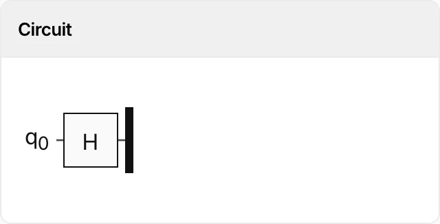
A qubit in superposition carries weights on both answers instead of holding one of them, and its answer is not fixed until the moment it is measured. Lesson 1 built a circuit with a certain answer; this one builds a circuit of that uncertain kind, and reads it 1,000 times at a go to see what that means.
The gate that does it is the Hadamard, h in Qiskit: one line of code and one idea.
Half and half, until you look
Start with an ordinary bit. It holds a 0 or a 1. If you have not looked at it you do not know which, but it is already one or the other, and looking only tells you which one it was.
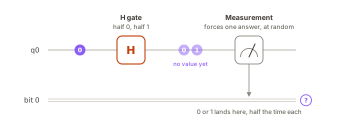
A qubit after a Hadamard gate is not a bit you have not looked at. Before the measurement there is no value in it to find. What it carries instead is a weight on each outcome, equal here, so each answer is equally likely. That state, weights on both answers at once, is a superposition.
The measurement is the step that turns those weights into one answer. Run the circuit again and the answer can come out the other way. A quantum program returns a tally for that reason: one answer cannot pin the weights down, and a thousand answers can.
Weights are more than odds. A weight has a size, which sets how likely its answer is: the share of shots that read an answer is its weight's size squared, so two equal weights of about 0.7 give shares of one half each.
A weight also has a sign, which never shows in a tally on its own.
It shows when another gate acts on the weights before the measurement, because gates transform the weights, sign included. The last assignment in this lesson is the first place it matters.
The Hadamard gate
Takes a qubit at 0 and leaves it weighted evenly between 0 and 1; takes a qubit at 1 and does the same with the sign of one weight flipped. Measure either and each answer is equally likely. Its own inverse: twice in a row and the qubit is back where it started.
The circuit, then the code
# 'backend' already exists when this runs: it is whatever you pick in the Run Experiment dialog.
from qiskit import QuantumCircuit
from qiskit.providers.jobstatus import JobStatus
import time
shots = 1000
qc = QuantumCircuit(1, 1)
1qc.h(0)
qc.measure(0, 0)
print(qc)
2job = backend.run(qc, shots=shots)
while job.status() not in (JobStatus.DONE, JobStatus.ERROR, JobStatus.CANCELLED):
time.sleep(5)
counts = job.result().get_counts()
print(counts)
for bits, n in sorted(counts.items()):
3 print(f"{bits}: {n:4d} {100 * n / shots:5.1f}% {'█' * (50 * n // shots)}")
- 1the Hadamard gate: half 0, half 1, and no value at all until it is measured
- 2one job per press of Run: press it again for another tally
- 3the share next to each bar, from lesson 1's second assignment
Two things changed in what the code does since lesson 1. The gate is h instead of x, and the bar loop prints each bar's share next to it, which was lesson 1's second assignment. Everything else, the qubit, the bit, the measurement, the job and backend, does the same as before.
Run the circuit, three presses
Three levels to keep apart. A shot is one execution of the circuit, start to finish. A job is one press: Run on Qollab, a choice in the dialog, then the dialog's Run. This listing's job holds 1,000 shots. The Playground files one job per press, so a second tally needs a second press.
Predict the tally. Then open the project, press Run on Qollab, choose IonQ Aria 1 under Remotely Run Simulators, and press Run. When the tally is in, note it and press twice more, choosing Aria 1 each time. Our first press took 17.9 seconds.
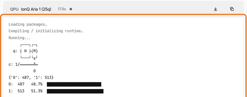
Our three presses on 15 September 2026, on the Aria 1 noise model, came back {'0': 487, '1': 513}, then {'0': 505, '1': 495}, then {'0': 511, '1': 489}. Three different splits from one circuit, none of them 500/500.
The ideal is exactly one half each, and a finite sample rarely lands on it. Even a perfect simulator gives 500 of 1,000 only about one run in forty.
Fork the project now, the way lesson 1 showed, so the edits below land in your own copy. The three assignments build on each other in order.
Assignment: one shot at a time
- In your fork, set
shots = 1and press three times, noting each tally. - Each dict can only be
{'0': 1}or{'1': 1}. Try to reconstruct the 50/50 split from your three dicts. - Write one sentence: what does one shot tell you about the weights inside the qubit?
Solution
One shot tells you which answer came out this time, not how likely it was. A single {'1': 1} is consistent with odds of 50/50 and with 99/1; it cannot tell them apart. The weights only appear across many shots, which is why a quantum program returns the tally rather than one answer.
Why the split is hardly ever exactly half
A fair split measured 1,000 times is a sample, and samples scatter. The expected count of 1s is 500. The typical distance from it, the standard deviation, is the square root of 1,000 times one half times one half, about 16 shots. Nineteen runs in twenty land within twice that, between about 468 and 532.
The same arithmetic at other sizes gives the rule for choosing a shot count. At 100 shots the scatter is 5 shots, which is 5% of the sample. At 10,000 it is 50 shots, which is half a percent.
Multiplying the shots by a hundred divides the scatter, as a share, by ten. Precision grows with the square root of the shot count, not with the count.
The weights inside the qubit never change between presses. What changes is the sample, and a bigger sample estimates the same weights more tightly. Lesson 1's noise tail was the same lesson from the other side. There the rare event was noise; here the scatter is built into a fair split.
Assignment: make the split move
- Set
shots = 100. Before you run, write down the band you expect the count of1s to land in: the expected count, 50, plus or minus twice the scatter, where the scatter is the square root of the shot count times one half. That gives 40 to 60. - Run, and note whether the count landed inside the band. Read the dict for the count and the Probabilities panel for the share.
- Set
shots = 10000and work out its band the same way. - Run, and note whether the count landed inside it.
One press cannot prove the rule. It can only land inside or outside the band it predicts, and nineteen presses in twenty land inside.
Solution
At 10,000 shots the scatter is 50, so the band is 4,900 to 5,100: within a percentage point of half. At 100 shots the band is 40 to 60: within ten points. Either press can miss its band about once in twenty; a miss is not a contradiction, it is the one in twenty.
The rule to keep is the shape of the bands: a hundred times the shots buys ten times the precision, never a hundred.
A superposition is not a hidden coin
Everything in the tally so far looks like a coin: one press, one answer, and no way to predict it. Suppose the qubit after one Hadamard were secretly a 0 or secretly a 1, and the measurement merely revealed it.
The gate row gives the test. The Hadamard spreads a qubit at 0 evenly, and it spreads a qubit at 1 evenly too. So if the qubit really held a hidden value, a second Hadamard would spread that value out again. The tally after two Hadamards would be half and half, just like after one.
Assignment: two Hadamards in a row
- Set
shotsback to1000. - Add a second
qc.h(0)directly under the first, before the measurement. - Write down two predictions: half and half, from the hidden-coin argument above, and the gate row's answer, its own inverse.
- Decide which you believe, then run.
Solution
Every shot reads 0, bar a few stray 1s from the noise model. The hidden coin predicted half and half and was wrong.
qc = QuantumCircuit(1, 1)
qc.h(0)
qc.h(0)
qc.measure(0, 0)
The Hadamard is its own inverse because the weights carry signs. After one Hadamard the two weights are equal in size and share a sign. A hidden 1 would have given equal sizes with opposite signs: the same tally, a different state.
The second Hadamard reads the signs. It adds the weights that agree and cancels the ones that disagree, and for the shared-sign state everything collects on 0. Lesson 5 is built on that step.
The Hadamard gave one qubit two possible answers. The next lesson adds a second qubit and a gate that acts on both, and the answers stop being independent of each other.
Stay in the loop.
Get the latest tutorials, demos, and project showcases straight to your inbox. No noise, just the good stuff.
On this page