Rabi Oscillations: Visualizing Excited-State Probability
A primer on the quantum dynamics of a driven two-level system, visualizing excited-state probability under the rotating-wave approximation (RWA).
About the author
Republished with the author's permission from the original notebook and shared under CC-BY-4.0. The text, code, and figures below are Onri's, as published.
This notebook provides a primer on the quantum dynamics of a driven two-level system by visualizing the excited-state probability under the rotating-wave approximation (RWA). The model treats a qubit as an ideal two-state system driven by a classical microwave tone. This formulation maps the probability of measuring the excited state as a function of drive frequency and pulse duration. The central computational object is the probability surface
where denotes the applied drive frequency and denotes the microwave pulse duration. The notebook renders this probability surface with two-dimensional heatmaps, three-dimensional surfaces, one-dimensional cross sections, and Fast Fourier transform (FFT) spectrograms. Fourier analysis exposes the generalized Rabi frequency as a theoretical ridge in the frequency domain, which connects the time-domain quantum oscillation to its spectral structure.
Nomenclature and Definitions
The following table defines the physical and mathematical quantities that recur throughout the visualization workflow.
| Symbol or Term | Meaning |
|---|---|
| Ground state of the qubit | |
| Excited state of the qubit | |
| Quantum state vector in a two-dimensional Hilbert space | |
| Complex probability amplitudes for and | |
| Probability of measuring the qubit in the excited state | |
| Natural transition frequency of the qubit | |
| Applied drive frequency | |
| Angular transition frequency, | |
| Angular drive frequency, | |
| On-resonance Rabi angular frequency | |
| On-resonance Rabi frequency in ordinary frequency units | |
| Drive detuning, | |
| Generalized Rabi angular frequency | |
| Generalized Rabi frequency, | |
| Pulse duration | |
| Phenomenological dephasing time used as an optional damping parameter | |
| RWA | Rotating-wave approximation |
| FFT | Fast Fourier transform |
Physical Model
A qubit can be modeled as a two-level quantum system with a ground state and an excited state . In the absence of a microwave drive, the energy splitting is
where the angular transition frequency is
The default configuration uses a transition frequency of
Applying a microwave drive with frequency induces coherent rotations between and . Exact resonance occurs when
At resonance, the drive produces ideal Rabi oscillations. Away from resonance, detuning changes the oscillation frequency and reduces the maximum achievable excited-state probability. This same two-level control structure appears across superconducting qubits, spin qubits, trapped ions, neutral atoms, and nitrogen-vacancy centers whenever a selected transition can be treated as an effective qubit.
Mathematical Foundation
The quantum state is a normalized vector in a two-dimensional Hilbert space,
where and are complex probability amplitudes. Normalization requires
The Born rule gives the probability of measuring the excited state,
Pauli matrices then provide a natural operator basis for the two-level system,
Within this representation, a driven two-level system behaves like a spin- particle precessing around an effective magnetic field. The drive strength supplies the transverse control component. Applied detuning supplies the longitudinal control component.
Rotating-Frame Hamiltonian
In the laboratory frame, a minimal semiclassical Hamiltonian for the driven qubit is
where is the drive angular frequency and is the on-resonance Rabi angular frequency. The computational model specifies the drive strength using in MHz. Transforming into a frame rotating at the drive frequency and applying the rotating-wave approximation gives the effective time-independent Hamiltonian
with detuning
This Hamiltonian describes precession around an effective control axis with components proportional to and . The transverse component drives population transfer. A longitudinal component tilts the rotation axis away from the resonant direction.
Excited-State Probability
The simulation assumes that the qubit begins in the ground state . Evolving under the RWA Hamiltonian, the probability of occupying the excited state after pulse duration is
where
is the generalized Rabi angular frequency. The amplitude coefficient
sets the maximum possible population transfer. At exact resonance, , so
Full population inversion is achievable in the ideal resonant model. For any nonzero detuning, the coefficient falls below one, so the state generally cannot reach unit excited-state probability.
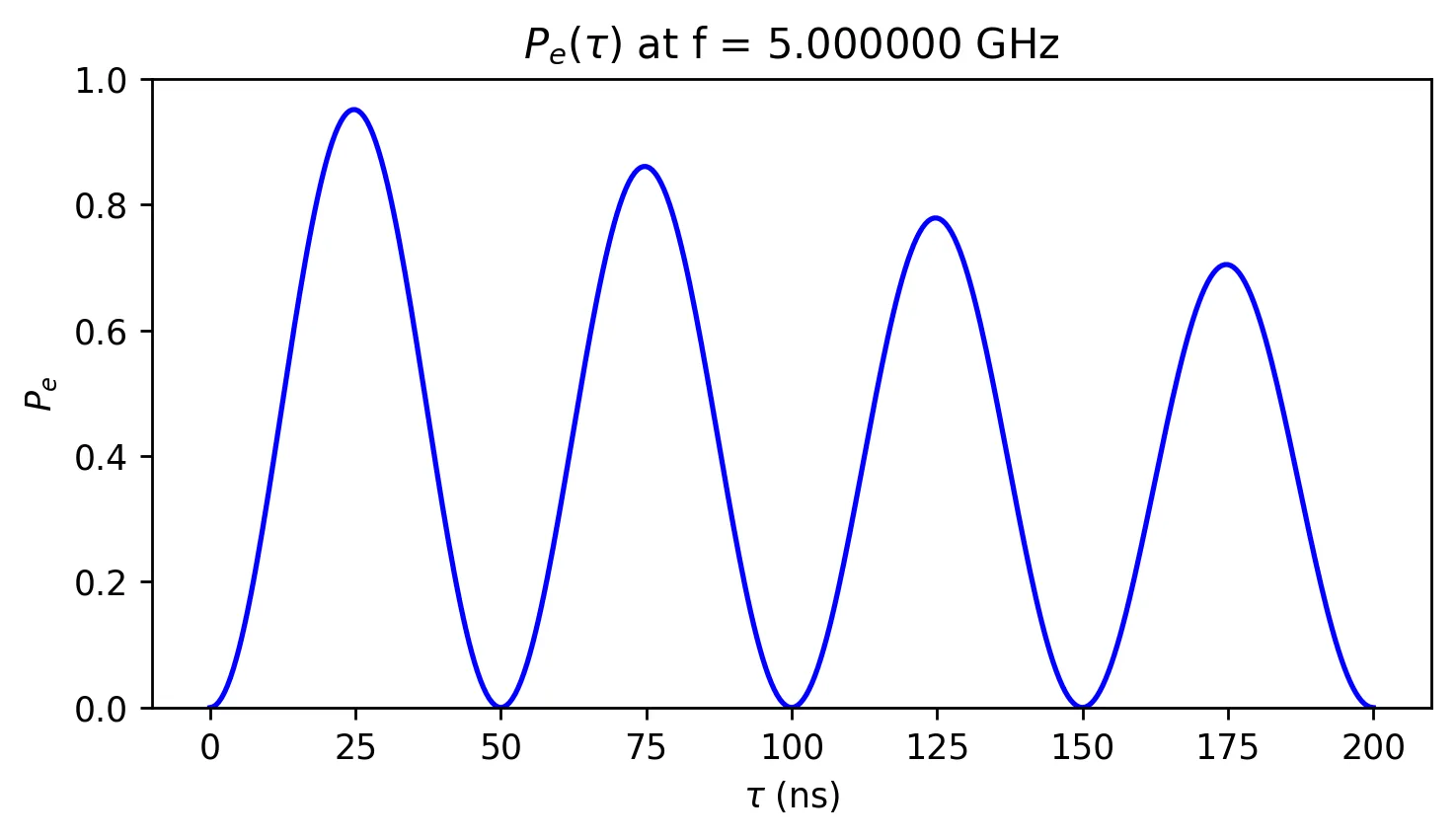
At resonance, the excited-state probability simplifies to
The pulse duration required for ideal population inversion defines the standard -pulse time,
Given the default drive strength
the ideal -pulse time is
A full period of the resonant excited-state probability oscillation is
For the same default drive strength, the full temporal period is
Phenomenological Dephasing
The computational model includes an optional phenomenological damping factor,
This exponential envelope attenuates the plotted Rabi fringes as pulse duration increases. The factor is a compact visualization device for contrast decay. A rigorous open-quantum-system treatment would require a density matrix model with relaxation channels, dephasing channels, finite temperature effects, shaped pulse envelopes, and stochastic dynamics. The default dephasing parameter is
Setting T2STAR_NS = None disables the phenomenological damping factor.
Detuning and Generalized Rabi Frequency
Detuning quantifies the spectral mismatch between the applied drive and the natural qubit transition,
Expressed in ordinary frequency units, the generalized Rabi frequency is
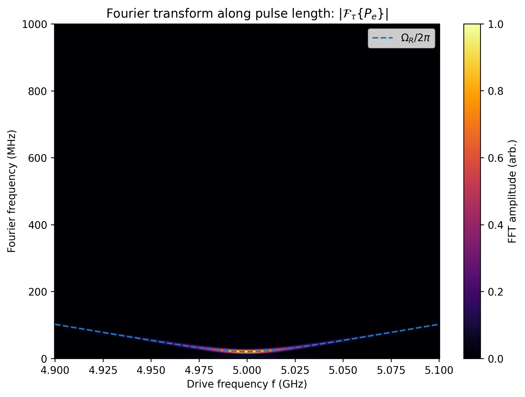
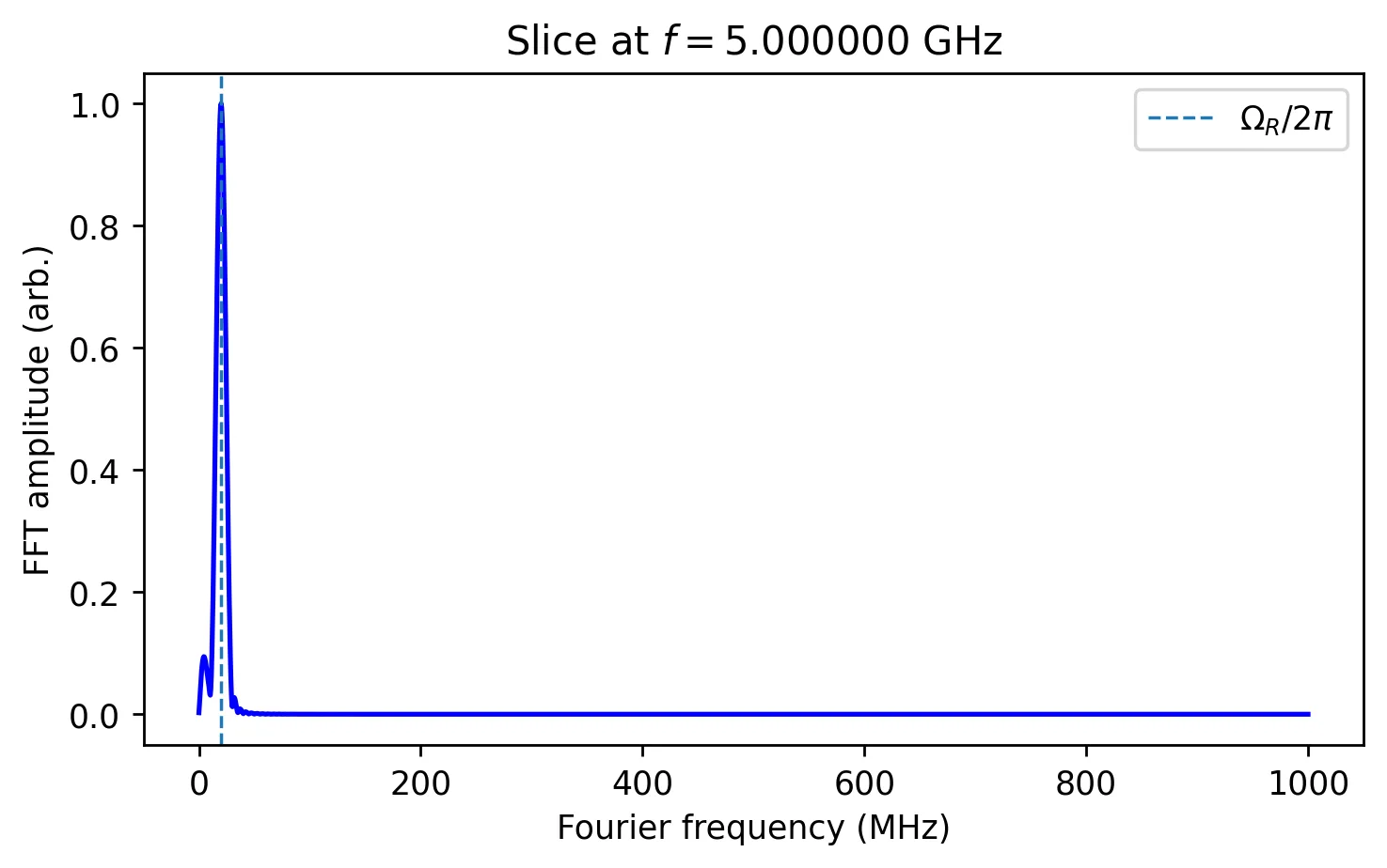
This expression explains the ridge visible in the Fourier-domain heatmap. At resonance, the generalized frequency equals the applied drive strength,
As the system moves away from resonance, increases symmetrically with . The oscillations accelerate along the pulse-duration axis, and the maximum achievable excited-state probability decreases. This tradeoff is the defining visual signature of detuned Rabi dynamics.
Quantum Information Interpretation
In quantum information language, a calibrated resonant Rabi pulse implements a single-qubit rotation. At exact resonance, the effective Hamiltonian is proportional to , so the microwave pulse implements
where
A calibrated resonant -pulse enacts
which corresponds to a quantum gate up to a global phase. A resonant -pulse prepares a balanced coherent superposition,
with a phase convention set by the microwave drive phase.
Detuning changes the rotation axis so it is no longer purely transverse. The unitary can be written as
where
This representation shows that detuning increases the rotation rate and tilts the control axis. Under this idealized model, the qubit still evolves coherently, although the trajectory generally misses the pure excited-state pole.
Bloch-Sphere Interpretation
A Bloch sphere maps any pure qubit state to a unit vector in three-dimensional space. Ground and excited states occupy opposite poles. Equal-amplitude coherent superpositions lie on the equator.
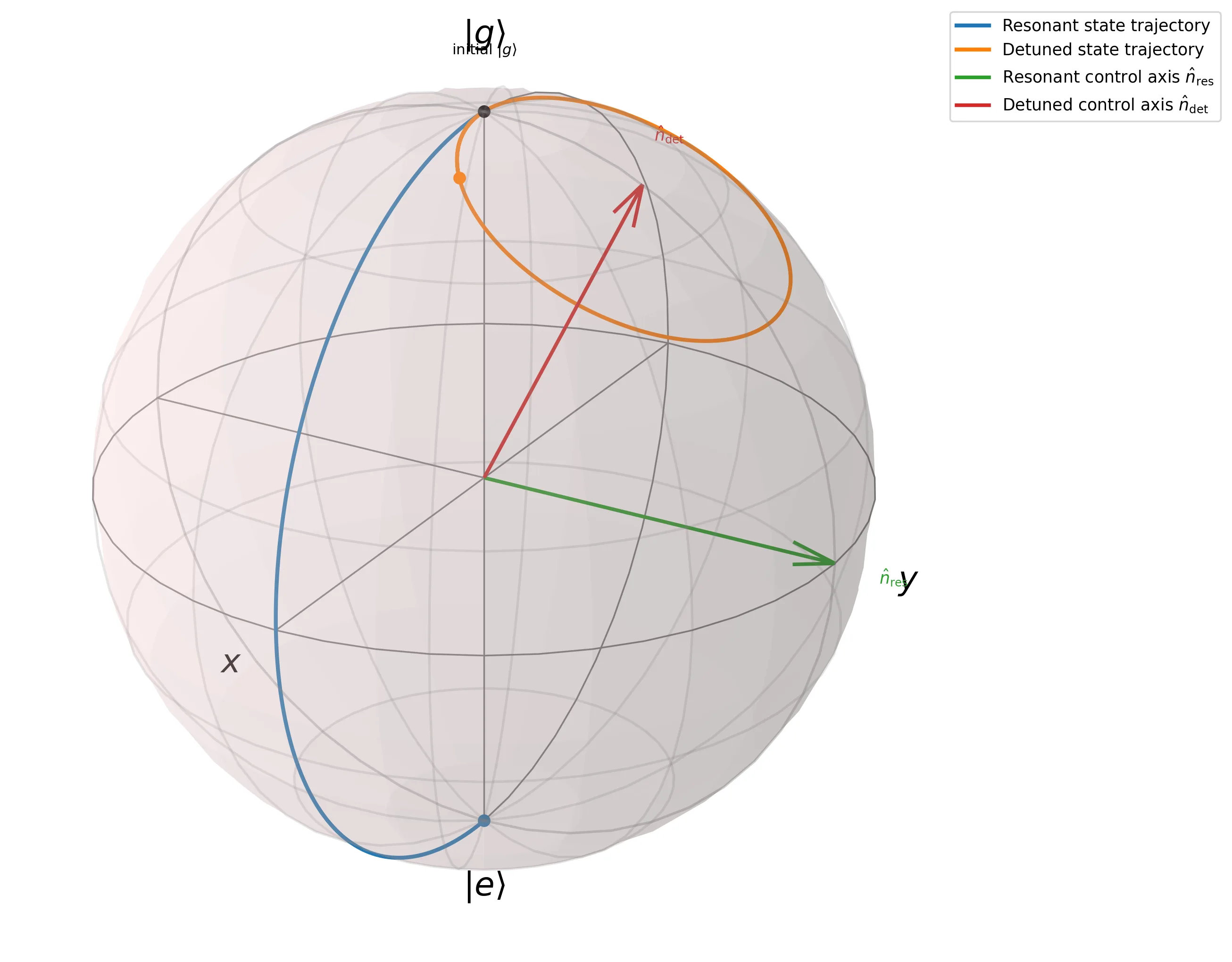
A resonant microwave drive rotates the Bloch vector around a transverse axis. Starting from , a properly timed -pulse moves the state to the excited-state pole. A -pulse moves the state to the equator, where the ground-state and excited-state measurement probabilities are equal.
Detuning tilts the rotation axis toward the -axis. The state vector then precesses around the tilted axis and generally fails to reach the excited-state pole. This geometric picture explains the amplitude coefficient
As grows, the rotation axis becomes more longitudinal, the oscillation frequency increases, and the maximum excited-state population decreases.
Fourier Analysis Dynamics
The spectral analysis computes a real Fast Fourier transform along the pulse-duration axis. For each sampled drive frequency , the trace is treated as a time-domain signal. The spectral amplitude is
This probability expression contains a squared sinusoid. Using the identity
shows that the dominant oscillatory spectral component appears at the generalized frequency
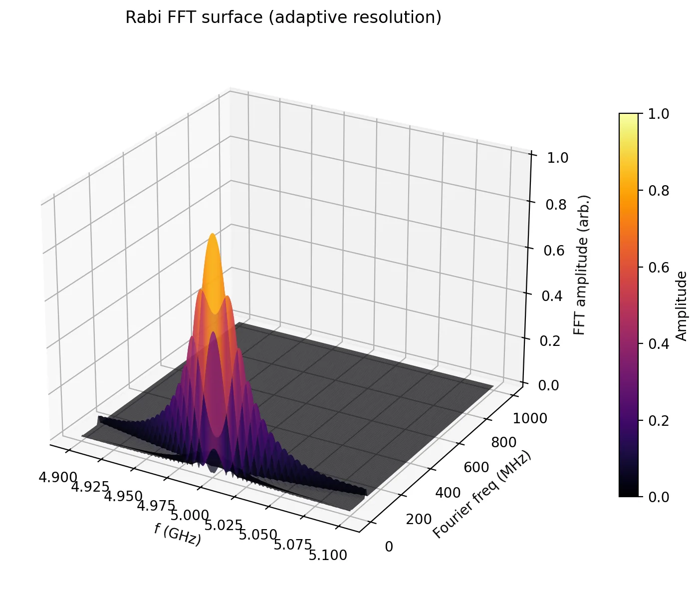
The computational workflow subtracts the mean signal along the pulse-duration axis, applies a Hann window to reduce spectral leakage, uses zero-padding to smooth the displayed Fourier grid, and overlays the exact generalized Rabi ridge on the Fourier heatmap. Zero-padding improves visual interpolation of the plotted spectrum, although the physical frequency resolution remains set by the sampled temporal window.
Computational Methodology
The notebook uses a deterministic closed-form workflow, so it does not require numerical time stepping of the Schrödinger equation. It defines a drive-frequency grid in GHz and a pulse-duration grid in ns, then converts both to SI units. From a dense two-dimensional mesh over and , the workflow computes the detuning , evaluates the generalized Rabi angular frequency , and calculates the analytic excited-state probability
The routine optionally applies the damping envelope and clips the result to the physical interval
Finally, the output is rendered as heatmaps, three-dimensional surfaces, one-dimensional slices, and Fourier-domain spectra. Standard scientific Python libraries provide the numerical arrays, visualization routines, and optional interactive rendering tools.
Graphical Interpretation
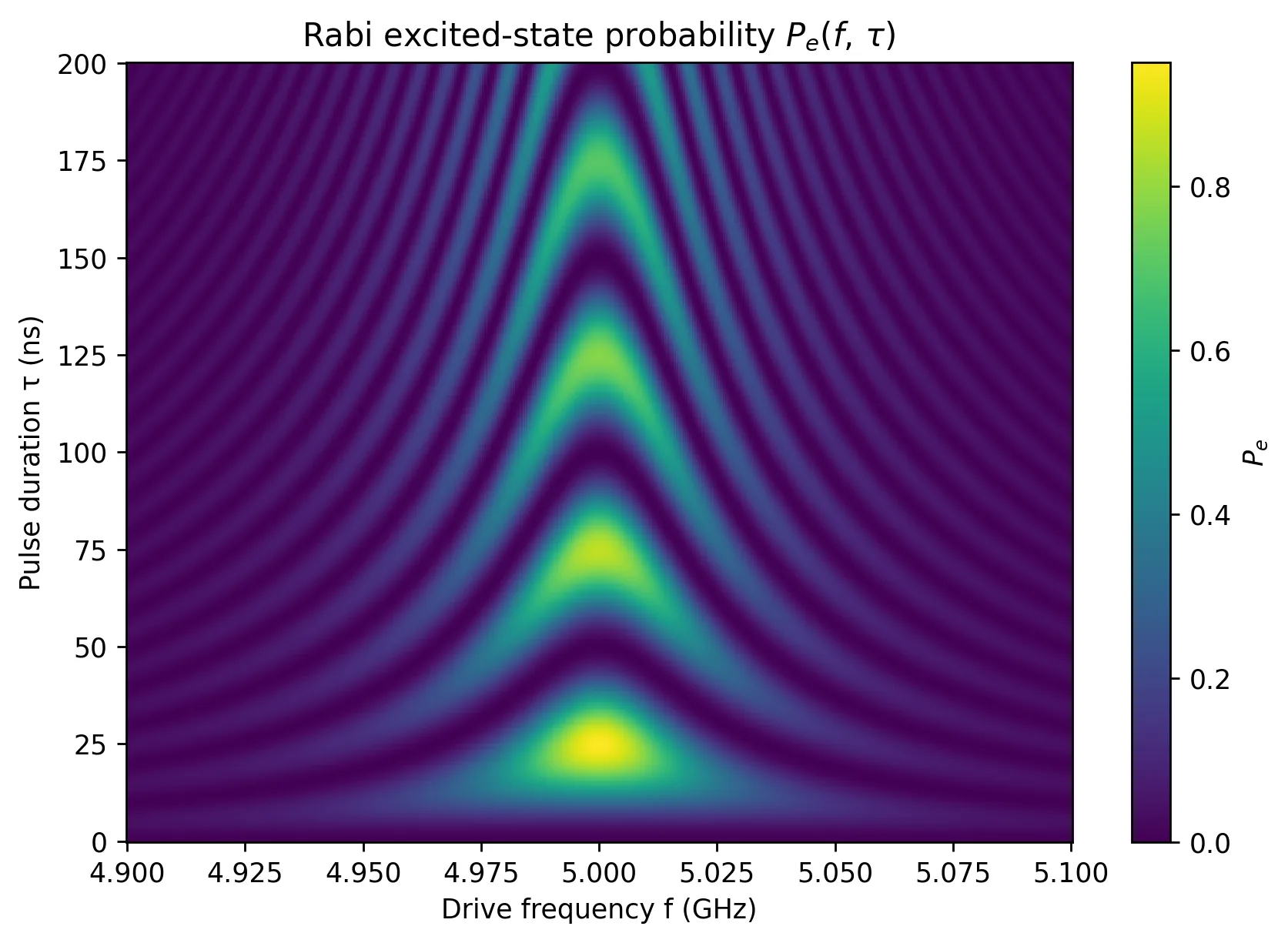
The heatmap shows the predicted probability of detecting the qubit in the excited state after applying a control pulse. Its horizontal axis gives the applied drive frequency. The vertical axis gives the pulse duration. Brighter regions indicate higher excited-state probability.
The resonant interaction region appears near
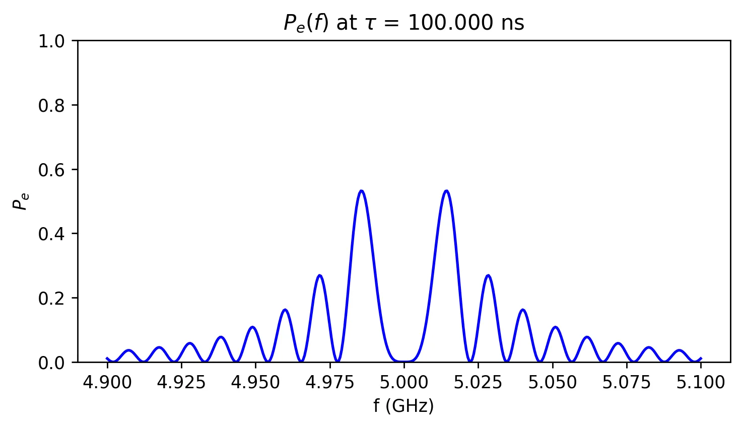
At resonance, contrast is maximal and the pulse duration alone sets the rotation angle. With the default drive strength , the ideal resonant maxima appear near
before the optional phenomenological damping factor is applied.
Off resonance, the fringes show lower contrast and faster temporal oscillations. This behavior follows from the generalized Rabi frequency , which increases with detuning, and from the amplitude coefficient , which decreases with detuning.
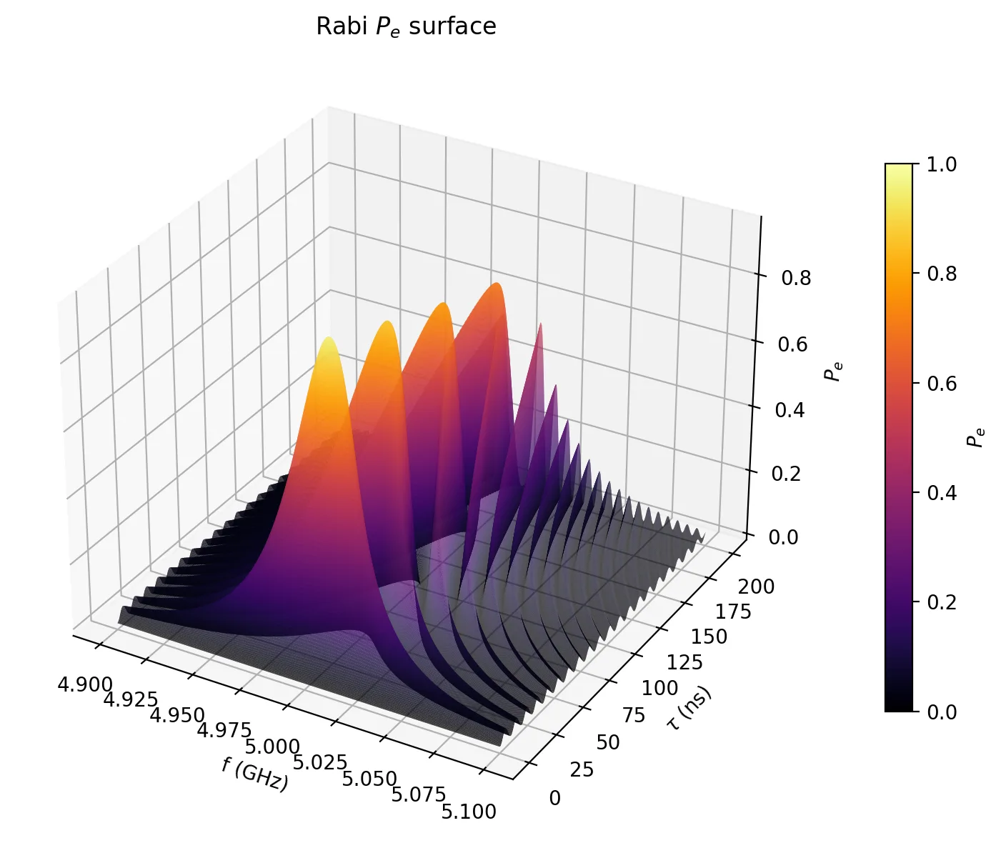
The three-dimensional surface plot represents the same probability data as a height field. This view emphasizes the central resonant ridge and the suppressed off-resonant oscillations. Cross-section plots isolate one-dimensional behavior. A fixed-frequency slice shows how probability evolves with pulse duration. At a fixed duration, a complementary slice shows how probability changes across the drive-frequency sweep.
The FFT heatmap characterizes the oscillation-frequency content of . An overlaid theoretical curve follows
Primary Modeling Assumptions
This notebook is an idealized mathematical physics visualization designed for conceptual clarity and calibration intuition.
| Assumption | Implication |
|---|---|
| Two-level truncation | The simulated model includes only and . |
| Classical drive | The microwave field is prescribed externally instead of quantized as a field mode. |
| Rotating-wave approximation | Fast counter-rotating terms are omitted. |
| Square pulse | The drive is assumed to turn on and off instantaneously. |
| Uniform drive amplitude | The parameter remains constant across the frequency sweep. |
| Optional damping envelope | The parameter enters as a simple exponential contrast envelope. |
| No explicit relaxation | Energy decay from to is omitted. |
| No higher-state leakage | Higher levels, including a transmon state, are excluded. |
| No AC Stark shift | Drive-induced transition-frequency shifts are excluded. |
| No Bloch-Siegert shift | Counter-rotating corrections are excluded. |
| No experimental readout model | Assignment errors and finite signal-to-noise effects are omitted. |
| No pulse-envelope shaping | Gaussian, DRAG, cosine, and hardware-specific envelopes are omitted. |
A hardware-accurate superconducting-qubit simulation requires additional structure, including anharmonic multilevel dynamics, calibrated microwave pulse envelopes, drive phase control, amplitude-dependent frequency shifts, finite thermal populations, leakage channels, and measurement infidelity modeled with density matrix dynamics.
Notebook Control Knobs
The first code section centralizes the main physical and numerical parameters for direct adjustment.
| Parameter | Default | Meaning |
|---|---|---|
F0_GHZ | 5.000 | Qubit transition frequency in GHz |
OMEGA_ONRESONANCE_MHZ | 20.0 | On-resonance Rabi rate in MHz |
FREQ_MIN_GHZ | 4.90 | Minimum swept drive frequency in GHz |
FREQ_MAX_GHZ | 5.10 | Maximum swept drive frequency in GHz |
N_FREQ | 401 | Number of drive-frequency samples |
DUR_MIN_NS | 0.0 | Minimum pulse duration in ns |
DUR_MAX_NS | 200.0 | Maximum pulse duration in ns |
N_DUR | 401 | Number of pulse-duration samples |
T2STAR_NS | 500.0 | Optional damping time in ns, with None disabling damping |
Additional cross-section plotting cells expose localized slice controls.
| Parameter | Default | Meaning |
|---|---|---|
F_CROSS_GHZ | 5.000 | Drive-frequency slice used to plot |
T_CROSS_NS | 100.0 | Pulse-duration slice used to plot |
Separate FFT processing controls support spectral analysis.
| Parameter | Default | Meaning |
|---|---|---|
FFT_PAD | 8 | Zero-padding factor used in the Fourier transform |
WINDOW | "hann" | Window function applied along the pulse-duration axis |
DETREND_MEAN | True | Flag that subtracts the mean before the FFT |
AMP_MODE | "magnitude" | Display mode for magnitude, power, or dB-scaled amplitude |
NORM_MODE | "global" | Normalization mode applied globally or per drive-frequency column |
FREQ_UNITS | "MHz" | Frequency units used on the Fourier-frequency axis |
Three-dimensional visualization cells add rendering controls for upsampling, colormaps, face-count limits, and viewing angles. These settings change the appearance of the rendered figures while preserving the analytic probability model.
# @title Install dependencies
import sys
%pip -q install pyvista pythreejs trame
# @title Controls & imports
import math
from typing import Optional, Tuple
import numpy as np
import matplotlib.pyplot as plt
import pandas as pd

try:
    import pyvista as pv  # optional; only for 3D interactive
    PV_AVAILABLE = True
except Exception:
    PV_AVAILABLE = False

plt.rcParams['figure.dpi'] = 250
plt.rcParams['axes.grid'] = False

# ---------- Control knobs ----------
F0_GHZ: float = 5.000        # Qubit transition freq f0 [GHz]
OMEGA_ONRESONANCE_MHZ: float = 20.0  # Ω/2π on-resonance [MHz]
FREQ_MIN_GHZ: float = 4.90   # Sweep min f [GHz]
FREQ_MAX_GHZ: float = 5.10   # Sweep max f [GHz]
N_FREQ: int = 401            # # of frequency points
DUR_MIN_NS: float = 0.0      # Sweep min duration τ [ns]
DUR_MAX_NS: float = 200.0    # Sweep max duration τ [ns]
N_DUR: int = 401             # # of duration points
T2STAR_NS: Optional[float] = 500.0  # None to disable exp(-τ/T2*)

print('Controls loaded.')
Controls loaded.
def rabi_probability(
    f_ghz: np.ndarray,
    tau_ns: np.ndarray,
    f0_ghz: float,
    omega_onres_mhz: float,
    t2star_ns: Optional[float] = None,
) -> np.ndarray:
    """Excited-state probability on a 2D grid (f, τ), under RWA.

    Args:
        f_ghz: 1D array of drive frequencies [GHz].
        tau_ns: 1D array of pulse durations [ns].
        f0_ghz: Qubit frequency on resonance [GHz].
        omega_onres_mhz: On-resonance Rabi rate Ω/2π [MHz].
        t2star_ns: Optional T2* [ns]; multiplies exp(−τ/T2*).

    Returns:
        2D array P_e with shape (len(tau_ns), len(f_ghz)).
    """
    two_pi = 2.0 * math.pi
    f = f_ghz * 1e9
    f0 = f0_ghz * 1e9
    tau = tau_ns * 1e-9
    omega = two_pi * omega_onres_mhz * 1e6  # rad/s

    F, TAU = np.meshgrid(f, tau, indexing='xy')
    Delta = two_pi * (F - f0)               # rad/s
    Omega_R = np.sqrt(omega**2 + Delta**2)

    with np.errstate(divide='ignore', invalid='ignore'):
        amp = (omega / Omega_R) ** 2
        phase = 0.5 * Omega_R * TAU
        Pe = amp * np.sin(phase) ** 2

    if t2star_ns is not None and t2star_ns > 0.0:
        decay = np.exp(-TAU / (t2star_ns * 1e-9))
        Pe = Pe * decay

    return np.clip(Pe, 0.0, 1.0)
freq_ghz = np.linspace(FREQ_MIN_GHZ, FREQ_MAX_GHZ, N_FREQ)
dur_ns = np.linspace(DUR_MIN_NS, DUR_MAX_NS, N_DUR)
Pe = rabi_probability(freq_ghz, dur_ns, F0_GHZ, OMEGA_ONRESONANCE_MHZ, T2STAR_NS)
print('Grid shape (τ × f):', Pe.shape)
Grid shape (τ × f): (401, 401)
controls_table = pd.DataFrame(
    [
        ['f0 (GHz)', F0_GHZ],
        ['Ω/2π on-res (MHz)', OMEGA_ONRESONANCE_MHZ],
        ['f sweep min (GHz)', FREQ_MIN_GHZ],
        ['f sweep max (GHz)', FREQ_MAX_GHZ],
        ['N_f', N_FREQ],
        ['τ sweep min (ns)', DUR_MIN_NS],
        ['τ sweep max (ns)', DUR_MAX_NS],
        ['N_τ', N_DUR],
        ['T2* (ns; None=off)', T2STAR_NS],
    ],
    columns=['Parameter', 'Value']
)
controls_table
Parameter  Value
0            f0 (GHz)    5.0
1   Ω/2π on-res (MHz)   20.0
2   f sweep min (GHz)    4.9
3   f sweep max (GHz)    5.1
4                 N_f  401.0
5    τ sweep min (ns)    0.0
6    τ sweep max (ns)  200.0
7                 N_τ  401.0
8  T2* (ns; None=off)  500.0
fig, ax = plt.subplots(figsize=(7, 5))
c = ax.pcolormesh(freq_ghz, dur_ns, Pe, shading='auto')
cb = fig.colorbar(c, ax=ax, label=r'$P_e$')
ax.set_xlabel('Drive frequency f (GHz)')
ax.set_ylabel('Pulse duration τ (ns)')
ax.set_title('Rabi excited-state probability $P_e(f,\\,\\tau)$')
fig.tight_layout()
plt.show()
# @title Cell: QuTiP Bloch sphere with labeled Rabi-control axes
"""Render labeled Bloch-sphere trajectories for resonant and detuned drives."""

import importlib.util
import subprocess
import sys

# -------------------------------------------------------------------------
# Control knobs
# -------------------------------------------------------------------------
INSTALL_BLOCH_DEPENDENCIES = True

BLOCH_REQUIRED_PACKAGES = {
    "numpy": "numpy",
    "matplotlib": "matplotlib",
    "scipy": "scipy",
    "qutip": "qutip",
}

BLOCH_F0_GHZ = globals().get("F0_GHZ", 5.000)
BLOCH_OMEGA_ONRESONANCE_MHZ = globals().get(
    "OMEGA_ONRESONANCE_MHZ",
    20.0,
)

BLOCH_RESONANT_DETUNING_MHZ = 0.0
BLOCH_DETUNED_DETUNING_MHZ = 40.0

# Use None to automatically plot one resonant pi pulse.
BLOCH_DURATION_NS = None

BLOCH_NUM_TIME_POINTS = 300
BLOCH_FIGSIZE = (8.8, 7.8)
BLOCH_DPI = 250
BLOCH_VIEW = [-60, 25]

BLOCH_SHOW_CONTROL_AXIS_ARROWS = True
BLOCH_SHOW_ARROW_TIP_LABELS = True
BLOCH_SHOW_ENDPOINT_MARKERS = True
BLOCH_SHOW_LEGEND = True
BLOCH_PRINT_SUMMARY = True

COLOR_RESONANT_TRAJECTORY = "tab:blue"
COLOR_DETUNED_TRAJECTORY = "tab:orange"
COLOR_RESONANT_AXIS = "tab:green"
COLOR_DETUNED_AXIS = "tab:red"
COLOR_INITIAL_STATE = "black"

TRAJECTORY_LINEWIDTH = 2.4
CONTROL_AXIS_LINEWIDTH = 2.2
ENDPOINT_MARKER_SIZE = 45
ARROW_LENGTH_RATIO = 0.12
ARROW_LABEL_SCALE = 1.16

LEGEND_LOCATION = "upper left"
LEGEND_BBOX_TO_ANCHOR = (1.02, 1.02)


def package_is_available(package_name: str) -> bool:
    """Return True when a package can be imported."""
    return importlib.util.find_spec(package_name) is not None


def install_missing_packages(
    required_packages: dict[str, str],
) -> None:
    """Install missing notebook packages using uv pip with a pip fallback."""
    if not INSTALL_BLOCH_DEPENDENCIES:
        return

    missing_package_names = [
        pip_name
        for import_name, pip_name in required_packages.items()
        if not package_is_available(import_name)
    ]

    if not missing_package_names:
        return

    try:
        subprocess.run(
            [sys.executable, "-m", "pip", "install", "-q", "uv"],
            check=True,
        )
        subprocess.run(
            [
                sys.executable,
                "-m",
                "uv",
                "pip",
                "install",
                "--system",
                "-q",
                *missing_package_names,
            ],
            check=True,
        )
    except (subprocess.CalledProcessError, FileNotFoundError):
        subprocess.run(
            [
                sys.executable,
                "-m",
                "pip",
                "install",
                "-q",
                *missing_package_names,
            ],
            check=True,
        )


install_missing_packages(BLOCH_REQUIRED_PACKAGES)

import matplotlib.pyplot as plt
import numpy as np
import qutip as qt
from matplotlib.lines import Line2D

try:
    from IPython import get_ipython

    ipython = get_ipython()
    if ipython is not None:
        ipython.run_line_magic("matplotlib", "inline")
except ImportError:
    pass

plt.rcParams.update(
    {
        "figure.dpi": BLOCH_DPI,
    }
)


def get_pi_pulse_duration_ns(omega_onresonance_mhz: float) -> float:
    """Return the resonant pi-pulse duration in nanoseconds."""
    return 1.0e3 / (2.0 * omega_onresonance_mhz)


def solve_rwa_bloch_trajectory(
    detuning_mhz: float,
    duration_ns: float,
    num_time_points: int,
) -> dict[str, np.ndarray | float]:
    """Solve the RWA two-level trajectory and return Bloch observables."""
    omega_rad_s = 2.0 * np.pi * BLOCH_OMEGA_ONRESONANCE_MHZ * 1.0e6
    delta_rad_s = 2.0 * np.pi * detuning_mhz * 1.0e6
    omega_generalized_rad_s = np.hypot(omega_rad_s, delta_rad_s)

    time_s = np.linspace(0.0, duration_ns * 1.0e-9, num_time_points)

    ground_state = qt.basis(2, 0)
    excited_state = qt.basis(2, 1)
    excited_projector = excited_state * excited_state.dag()

    hamiltonian = 0.5 * (
        delta_rad_s * qt.sigmaz()
        + omega_rad_s * qt.sigmax()
    )

    result = qt.sesolve(
        hamiltonian,
        ground_state,
        time_s,
    )

    x_expectation = np.real(np.asarray(qt.expect(qt.sigmax(), result.states)))
    y_expectation = np.real(np.asarray(qt.expect(qt.sigmay(), result.states)))
    z_expectation = np.real(np.asarray(qt.expect(qt.sigmaz(), result.states)))

    excited_probability = np.real(
        np.asarray(qt.expect(excited_projector, result.states))
    )

    bloch_vectors = np.vstack(
        [
            x_expectation,
            y_expectation,
            z_expectation,
        ]
    )

    control_axis = np.array(
        [
            omega_rad_s / omega_generalized_rad_s,
            0.0,
            delta_rad_s / omega_generalized_rad_s,
        ]
    )

    return {
        "time_ns": time_s * 1.0e9,
        "vectors": bloch_vectors,
        "excited_probability": excited_probability,
        "control_axis": control_axis,
        "generalized_rabi_mhz": (
            omega_generalized_rad_s / (2.0 * np.pi * 1.0e6)
        ),
    }


def render_empty_bloch_sphere(
    bloch_sphere: qt.Bloch,
    fallback_figure: plt.Figure,
):
    """Render an empty QuTiP Bloch sphere and return its Matplotlib axis."""
    if hasattr(bloch_sphere, "render"):
        bloch_sphere.render()
    elif hasattr(bloch_sphere, "make_sphere"):
        bloch_sphere.make_sphere()
    else:
        bloch_sphere.show()

    axis = getattr(bloch_sphere, "axes", None)

    if axis is None and fallback_figure.axes:
        axis = fallback_figure.axes[-1]

    if axis is None:
        raise RuntimeError("Could not access the Matplotlib Bloch axis.")

    return axis


def draw_bloch_trajectory(
    axis,
    vectors: np.ndarray,
    color: str,
    label: str,
) -> None:
    """Draw a Bloch-vector trajectory on an existing 3D axis."""
    axis.plot(
        vectors[0],
        vectors[1],
        vectors[2],
        color=color,
        linewidth=TRAJECTORY_LINEWIDTH,
        label=label,
    )


def draw_endpoint_marker(
    axis,
    vector: np.ndarray,
    color: str,
    label: str,
) -> None:
    """Draw a marker at the final point of a Bloch trajectory."""
    axis.scatter(
        vector[0],
        vector[1],
        vector[2],
        color=color,
        s=ENDPOINT_MARKER_SIZE,
        depthshade=True,
        label=label,
    )


def draw_control_axis_arrow(
    axis,
    vector: np.ndarray,
    color: str,
    label: str,
) -> None:
    """Draw a normalized effective-control-axis arrow."""
    axis.quiver(
        0.0,
        0.0,
        0.0,
        vector[0],
        vector[1],
        vector[2],
        color=color,
        linewidth=CONTROL_AXIS_LINEWIDTH,
        arrow_length_ratio=ARROW_LENGTH_RATIO,
        normalize=False,
        label=label,
    )


def add_arrow_tip_label(
    axis,
    vector: np.ndarray,
    text: str,
    color: str,
) -> None:
    """Place a text label slightly beyond the arrow tip."""
    label_position = ARROW_LABEL_SCALE * vector

    axis.text(
        label_position[0],
        label_position[1],
        label_position[2],
        text,
        color=color,
        fontsize=10,
        ha="center",
        va="center",
    )


def add_initial_state_label(axis) -> None:
    """Label the initialized ground-state pole."""
    axis.scatter(
        0.0,
        0.0,
        1.0,
        color=COLOR_INITIAL_STATE,
        s=ENDPOINT_MARKER_SIZE,
        depthshade=True,
    )
    axis.text(
        0.0,
        0.0,
        1.16,
        r"initial $|g\rangle$",
        color=COLOR_INITIAL_STATE,
        fontsize=9,
        ha="center",
        va="center",
    )


if BLOCH_DURATION_NS is None:
    bloch_duration_ns = get_pi_pulse_duration_ns(
        BLOCH_OMEGA_ONRESONANCE_MHZ
    )
else:
    bloch_duration_ns = BLOCH_DURATION_NS

resonant_trajectory = solve_rwa_bloch_trajectory(
    detuning_mhz=BLOCH_RESONANT_DETUNING_MHZ,
    duration_ns=bloch_duration_ns,
    num_time_points=BLOCH_NUM_TIME_POINTS,
)

detuned_trajectory = solve_rwa_bloch_trajectory(
    detuning_mhz=BLOCH_DETUNED_DETUNING_MHZ,
    duration_ns=bloch_duration_ns,
    num_time_points=BLOCH_NUM_TIME_POINTS,
)

resonant_drive_ghz = (
    BLOCH_F0_GHZ
    + BLOCH_RESONANT_DETUNING_MHZ * 1.0e-3
)
detuned_drive_ghz = (
    BLOCH_F0_GHZ
    + BLOCH_DETUNED_DETUNING_MHZ * 1.0e-3
)

figure = plt.figure(figsize=BLOCH_FIGSIZE)

bloch = qt.Bloch(fig=figure)
bloch.view = BLOCH_VIEW
bloch.zlabel = [r"$|g\rangle$", r"$|e\rangle$"]
bloch.title = (
    "Bloch-sphere Rabi trajectories\n"
    rf"resonant $\Delta/2\pi={BLOCH_RESONANT_DETUNING_MHZ:.1f}$ MHz, "
    rf"detuned $\Delta/2\pi={BLOCH_DETUNED_DETUNING_MHZ:.1f}$ MHz"
)

bloch_axis = render_empty_bloch_sphere(
    bloch_sphere=bloch,
    fallback_figure=figure,
)

draw_bloch_trajectory(
    axis=bloch_axis,
    vectors=resonant_trajectory["vectors"],
    color=COLOR_RESONANT_TRAJECTORY,
    label="Resonant state trajectory",
)
draw_bloch_trajectory(
    axis=bloch_axis,
    vectors=detuned_trajectory["vectors"],
    color=COLOR_DETUNED_TRAJECTORY,
    label="Detuned state trajectory",
)

if BLOCH_SHOW_ENDPOINT_MARKERS:
    draw_endpoint_marker(
        axis=bloch_axis,
        vector=resonant_trajectory["vectors"][:, -1],
        color=COLOR_RESONANT_TRAJECTORY,
        label="Resonant final state",
    )
    draw_endpoint_marker(
        axis=bloch_axis,
        vector=detuned_trajectory["vectors"][:, -1],
        color=COLOR_DETUNED_TRAJECTORY,
        label="Detuned final state",
    )
    add_initial_state_label(bloch_axis)

if BLOCH_SHOW_CONTROL_AXIS_ARROWS:
    draw_control_axis_arrow(
        axis=bloch_axis,
        vector=resonant_trajectory["control_axis"],
        color=COLOR_RESONANT_AXIS,
        label=r"Resonant control axis $\hat{n}_{\mathrm{res}}$",
    )
    draw_control_axis_arrow(
        axis=bloch_axis,
        vector=detuned_trajectory["control_axis"],
        color=COLOR_DETUNED_AXIS,
        label=r"Detuned control axis $\hat{n}_{\mathrm{det}}$",
    )

if BLOCH_SHOW_ARROW_TIP_LABELS and BLOCH_SHOW_CONTROL_AXIS_ARROWS:
    add_arrow_tip_label(
        axis=bloch_axis,
        vector=resonant_trajectory["control_axis"],
        text=r"$\hat{n}_{\mathrm{res}}$",
        color=COLOR_RESONANT_AXIS,
    )
    add_arrow_tip_label(
        axis=bloch_axis,
        vector=detuned_trajectory["control_axis"],
        text=r"$\hat{n}_{\mathrm{det}}$",
        color=COLOR_DETUNED_AXIS,
    )

if BLOCH_SHOW_LEGEND:
    legend_handles = [
        Line2D(
            [0],
            [0],
            color=COLOR_RESONANT_TRAJECTORY,
            linewidth=TRAJECTORY_LINEWIDTH,
            label="Resonant state trajectory",
        ),
        Line2D(
            [0],
            [0],
            color=COLOR_DETUNED_TRAJECTORY,
            linewidth=TRAJECTORY_LINEWIDTH,
            label="Detuned state trajectory",
        ),
        Line2D(
            [0],
            [0],
            color=COLOR_RESONANT_AXIS,
            linewidth=CONTROL_AXIS_LINEWIDTH,
            label=r"Resonant control axis $\hat{n}_{\mathrm{res}}$",
        ),
        Line2D(
            [0],
            [0],
            color=COLOR_DETUNED_AXIS,
            linewidth=CONTROL_AXIS_LINEWIDTH,
            label=r"Detuned control axis $\hat{n}_{\mathrm{det}}$",
        ),
    ]

    bloch_axis.legend(
        handles=legend_handles,
        loc=LEGEND_LOCATION,
        bbox_to_anchor=LEGEND_BBOX_TO_ANCHOR,
        frameon=True,
        borderaxespad=0.0,
    )

plt.show()

if BLOCH_PRINT_SUMMARY:
    resonant_axis = resonant_trajectory["control_axis"]
    detuned_axis = detuned_trajectory["control_axis"]

    print("Bloch-sphere trajectory summary")
    print(f"Natural transition frequency f0: {BLOCH_F0_GHZ:.6f} GHz")
    print(f"Resonant drive frequency: {resonant_drive_ghz:.6f} GHz")
    print(f"Detuned drive frequency: {detuned_drive_ghz:.6f} GHz")
    print(f"On-resonance Rabi rate: {BLOCH_OMEGA_ONRESONANCE_MHZ:.3f} MHz")
    print(f"Plotted duration: {bloch_duration_ns:.3f} ns")
    print(
        "Resonant control axis n_res: "
        f"({resonant_axis[0]:.6f}, "
        f"{resonant_axis[1]:.6f}, "
        f"{resonant_axis[2]:.6f})"
    )
    print(
        "Detuned control axis n_det: "
        f"({detuned_axis[0]:.6f}, "
        f"{detuned_axis[1]:.6f}, "
        f"{detuned_axis[2]:.6f})"
    )
    print(
        "Resonant final excited-state probability: "
        f"{resonant_trajectory['excited_probability'][-1]:.6f}"
    )
    print(
        "Detuned final excited-state probability: "
        f"{detuned_trajectory['excited_probability'][-1]:.6f}"
    )
    print(
        "Detuned generalized Rabi frequency: "
        f"{detuned_trajectory['generalized_rabi_mhz']:.6f} MHz"
    )
Bloch-sphere trajectory summary
Natural transition frequency f0: 5.000000 GHz
Resonant drive frequency: 5.000000 GHz
Detuned drive frequency: 5.040000 GHz
On-resonance Rabi rate: 20.000 MHz
Plotted duration: 25.000 ns
Resonant control axis n_res: (1.000000, 0.000000, 0.000000)
Detuned control axis n_det: (0.447214, 0.000000, 0.894427)
Resonant final excited-state probability: 1.000000
Detuned final excited-state probability: 0.026264
Detuned generalized Rabi frequency: 44.721360 MHz
# --- High-resolution 3D surface with colormap & legend  ---
from mpl_toolkits.mplot3d import Axes3D
import numpy as np
import matplotlib.pyplot as plt

# Controls for surface quality and appearance
UPSAMPLE_FACTOR: int = 2           # 2=~4× more faces; try 3 for even smoother
SURFACE_CMAP: str = 'inferno'      # e.g., 'viridis', 'plasma', 'magma', 'inferno'
Z_MIN, Z_MAX = 0.0, 1.0            # clamp/normalize expected Pe range

# --- Bilinear upsampling (SciPy-free) ---
# 1) Upsample frequency axis for each fixed τ
freq_hi = np.linspace(freq_ghz.min(), freq_ghz.max(),
                      UPSAMPLE_FACTOR * (len(freq_ghz) - 1) + 1)
Pe_tau_f = np.empty((len(dur_ns), len(freq_hi)), dtype=float)
for i in range(len(dur_ns)):
    Pe_tau_f[i, :] = np.interp(freq_hi, freq_ghz, Pe[i, :])

# 2) Upsample τ axis for each fixed frequency
dur_hi = np.linspace(dur_ns.min(), dur_ns.max(),
                     UPSAMPLE_FACTOR * (len(dur_ns) - 1) + 1)
Pe_hi = np.empty((len(dur_hi), len(freq_hi)), dtype=float)
for j in range(len(freq_hi)):
    Pe_hi[:, j] = np.interp(dur_hi, dur_ns, Pe_tau_f[:, j])

# Mesh for plotting
F_hi, T_hi = np.meshgrid(freq_hi, dur_hi, indexing='xy')

# --- Plot ---
fig = plt.figure(figsize=(8, 6), dpi=200)
ax = fig.add_subplot(111, projection='3d')

surf = ax.plot_surface(
    F_hi, T_hi, Pe_hi,
    rstride=1, cstride=1,             # use every row/column (after upsampling)
    linewidth=0, antialiased=True,
    cmap=SURFACE_CMAP,
    vmin=Z_MIN, vmax=Z_MAX,
)

ax.set_xlabel('f (GHz)')
ax.set_ylabel(r'$\tau$ (ns)')
ax.set_zlabel(r'$P_e$')
ax.set_title('Rabi $P_e$ surface')

# Colorbar (legend for the colormap)
cb = fig.colorbar(surf, ax=ax, shrink=0.7, pad=0.08)
cb.set_label(r'$P_e$')

fig.tight_layout()
plt.show()
# @title Cross-sections
# Slicing controls
F_CROSS_GHZ: float = 5.000  # drive frequency slice [GHz]
T_CROSS_NS: float = 100.0   # duration slice [ns]

import numpy as np
import matplotlib.pyplot as plt

def _nearest_index(vec: np.ndarray, value: float, name: str) -> int:
    """Return nearest index to 'value' in 'vec'; clamp and notify if out of range."""
    vmin, vmax = float(vec.min()), float(vec.max())
    if value < vmin or value > vmax:
        print(f"[Note] {name}={value} is outside sweep; clamping to [{vmin}, {vmax}].")
        value = np.clip(value, vmin, vmax)
    return int(np.argmin(np.abs(vec - value)))

# --- Slice at f = F_CROSS_GHZ ---
j = _nearest_index(freq_ghz, F_CROSS_GHZ, "F_CROSS_GHZ")
Pe_vs_tau = Pe[:, j]

fig, ax = plt.subplots(figsize=(6, 3.5))
ax.plot(dur_ns, Pe_vs_tau, color='blue')
ax.set_xlabel(r'$\tau$ (ns)')
ax.set_ylabel(r'$P_e$')
# Avoid \text{}; mix math for symbols and plain text for units/values
ax.set_title(r'$P_e(\tau)$ at f = ' + f'{freq_ghz[j]:.6f} GHz')
ax.set_ylim(0.0, 1.0)
fig.tight_layout()
plt.show()

# --- Slice at τ = T_CROSS_NS ---
i = _nearest_index(dur_ns, T_CROSS_NS, "T_CROSS_NS")
Pe_vs_f = Pe[i, :]

fig, ax = plt.subplots(figsize=(6, 3.5))
ax.plot(freq_ghz, Pe_vs_f, color='blue')
ax.set_xlabel('f (GHz)')
ax.set_ylabel(r'$P_e$')
ax.set_title(r'$P_e(f)$ at $\tau$ = ' + f'{dur_ns[i]:.3f} ns')
ax.set_ylim(0.0, 1.0)
fig.tight_layout()
plt.show()
# @title FFT of Rabi oscillations along tau (controls + computation)
import numpy as np
import matplotlib.pyplot as plt

# -------- Control knobs (FFT & display) --------
FFT_PAD: int = 8                 # zero-padding factor (2, 4, 8, ...)
WINDOW: str = "hann"             # "hann", "boxcar"
DETREND_MEAN: bool = True        # subtract mean along τ before FFT
AMP_MODE: str = "magnitude"      # "magnitude" | "power" | "db"
NORM_MODE: str = "global"        # "global" | "per_f" (column-wise)
FREQ_UNITS: str = "MHz"          # "MHz" or "GHz" for Fourier axis

# -------- Helpers --------
def _make_window(n: int, kind: str) -> np.ndarray:
    if kind.lower() == "hann":
        return np.hanning(n)
    return np.ones(n, dtype=float)  # boxcar

def rfft_spectrogram(
    Pe: np.ndarray,
    dur_ns: np.ndarray,
    pad: int = 8,
    window: str = "hann",
    detrend_mean: bool = True,
    amp_mode: str = "magnitude",
    norm_mode: str = "global",
    freq_units: str = "MHz",
) -> tuple[np.ndarray, np.ndarray]:
    """Compute RFFT along τ for each drive frequency column of Pe(τ, f).

    Args:
        Pe: array of shape (N_tau, N_f) with excited-state probabilities.
        dur_ns: τ grid [ns], length N_tau, evenly spaced.
        pad: zero-padding factor (≥1).
        window: "hann" or "boxcar".
        detrend_mean: subtract column-wise mean before FFT.
        amp_mode: "magnitude", "power", or "db".
        norm_mode: "global" (single max) or "per_f" (each column scaled to its max).
        freq_units: "MHz" or "GHz" for the Fourier axis.

    Returns:
        f_fft: Fourier frequency axis [MHz or GHz] (length N_w),
        S:     2D nonnegative spectrogram (N_w, N_f).
    """
    Pe = np.asarray(Pe, float)
    dur_ns = np.asarray(dur_ns, float)
    assert Pe.shape[0] == dur_ns.size, "Pe must be shaped (N_tau, N_f)."

    # Uniform sampling assumption (true for np.linspace)
    dt = float(dur_ns[1] - dur_ns[0]) * 1e-9               # [s]
    n_tau = dur_ns.size
    nfft = int(2 ** int(np.ceil(np.log2(n_tau))) * max(1, pad))
    w = _make_window(n_tau, window)

    # Prepare output
    S_list = []
    X = Pe.copy()
    if detrend_mean:
        X = X - X.mean(axis=0, keepdims=True)
    X *= w[:, None]

    # Real FFT along τ (axis=0)
    Xf = np.fft.rfft(X, n=nfft, axis=0)                     # shape (N_w, N_f)
    f_fft_hz = np.fft.rfftfreq(nfft, d=dt)                  # [Hz]

    # Amplitude selection
    if amp_mode.lower() == "power":
        S = np.abs(Xf) ** 2
    else:
        S = np.abs(Xf)

    # Normalization
    if norm_mode.lower() == "per_f":
        col_max = np.maximum(S.max(axis=0, keepdims=True), 1e-15)
        S = S / col_max
    else:
        S = S / max(S.max(), 1e-15)

    if amp_mode.lower() == "db":
        S = 20.0 * np.log10(np.maximum(S, 1e-12))  # dB, clipped floor

    # Units
    if freq_units.upper() == "GHz":
        f_fft = f_fft_hz * 1e-9
    else:
        f_fft = f_fft_hz * 1e-6

    return f_fft, S

# Compute spectrogram with current grid
f_fft_axis, S_fft = rfft_spectrogram(
    Pe, dur_ns,
    pad=FFT_PAD,
    window=WINDOW,
    detrend_mean=DETREND_MEAN,
    amp_mode=AMP_MODE,
    norm_mode=NORM_MODE,
    freq_units=FREQ_UNITS,
)
print("FFT grid:", S_fft.shape, "| Fourier freq range:", f_fft_axis[0], "→", f_fft_axis[-1], FREQ_UNITS)
FFT grid: (2049, 401) | Fourier freq range: 0.0 → 999.9999999999999 MHz
# @title Theoretical Rabi ridge
import math
two_pi = 2.0 * math.pi
f0 = F0_GHZ * 1e9
delta_hz = two_pi * (freq_ghz*1e9 - f0)   # rad/s detuning
omega_onres = two_pi * OMEGA_ONRESONANCE_MHZ * 1e6  # rad/s
Omega_R = np.sqrt(omega_onres**2 + delta_hz**2)     # rad/s
ridge_hz = Omega_R / (2.0 * math.pi)                # Hz
if FREQ_UNITS.upper() == "GHz":
    ridge_axis = ridge_hz * 1e-9
else:
    ridge_axis = ridge_hz * 1e-6  # MHz
# @title 2D heatmap
fig, ax = plt.subplots(figsize=(7.5, 5.5))
im = ax.pcolormesh(freq_ghz, f_fft_axis, S_fft, shading="auto", cmap="inferno")
cb = fig.colorbar(im, ax=ax)
cb.set_label("FFT amplitude" + (" (dB)" if AMP_MODE.lower()=="db" else " (arb.)"))

ax.plot(freq_ghz, ridge_axis, "--", lw=1.5, label=r"$\Omega_R/2\pi$")
ax.set_xlabel("Drive frequency f (GHz)")
ax.set_ylabel(f"Fourier frequency ({FREQ_UNITS})")
ax.set_title("Fourier transform along pulse length: $|\\mathcal{F}_\\tau\\{P_e\\}|$")
ax.legend(loc="upper right")
fig.tight_layout()
plt.show()
# --- Adaptive high-res 3D surface ---
from mpl_toolkits.mplot3d import Axes3D
import numpy as np
import matplotlib.pyplot as plt

# ------ Control knobs ------
UPSAMPLE_F_FREQ: int = 3       # try 2–3; upsample the drive-frequency axis only
MAX_FACES: int = 300_000       # cap on triangles to avoid OOM / crashes (≈300k–500k is OK)
MIN_ROWS: int = 128            # keep at least this many Fourier-frequency rows
MAX_ROWS: int = 1024           # hard cap for rows to keep plotting fast

# Preserve global color limits so the legend stays consistent
vmin = float(np.nanmin(S_fft))
vmax = float(np.nanmax(S_fft))

# Shapes
n_rows, n_cols = S_fft.shape        # rows=Fourier freq (ν), cols=drive freq (f)

# 1) Upsample along the typically smaller axis (drive frequency) only
n_cols_up = min(UPSAMPLE_F_FREQ * (n_cols - 1) + 1, 1200)  # sensible upper bound
freq_hi = np.linspace(freq_ghz.min(), freq_ghz.max(), n_cols_up)

S_up_f = np.empty((n_rows, n_cols_up), dtype=float)
for i in range(n_rows):
    S_up_f[i, :] = np.interp(freq_hi, freq_ghz, S_fft[i, :])

# 2) Determine how many Fourier rows we can afford for MAX_FACES
# faces ≈ (n_rows_plot-1) * (n_cols_up-1)
n_rows_cap = int(MAX_FACES / max(n_cols_up - 1, 1)) + 1
n_rows_plot = int(np.clip(n_rows_cap, MIN_ROWS, min(MAX_ROWS, n_rows)))

# Down-sample ν-axis evenly to n_rows_plot
row_idx = np.linspace(0, n_rows - 1, n_rows_plot).astype(int)
f_fft_plot = f_fft_axis[row_idx]
S_final = S_up_f[row_idx, :]

# Mesh for plotting
F2_hi, FFOUR_hi = np.meshgrid(freq_hi, f_fft_plot, indexing="xy")

# 3) Plot (keeps 'inferno')
fig = plt.figure(figsize=(8, 6), dpi=200)
ax = fig.add_subplot(111, projection="3d")
surf = ax.plot_surface(
    F2_hi, FFOUR_hi, S_final,
    rstride=1, cstride=1,
    linewidth=0, antialiased=True,
    cmap="inferno",
    vmin=vmin, vmax=vmax
)

ax.set_xlabel("f (GHz)")
ax.set_ylabel(f"Fourier freq ({FREQ_UNITS})")
ax.set_zlabel("FFT amplitude" + (" (dB)" if AMP_MODE.lower() == "db" else " (arb.)"))
ax.set_title("Rabi FFT surface (adaptive resolution)")
fig.colorbar(surf, ax=ax, shrink=0.7, pad=0.08, label="Amplitude")

# A clearer default view
ax.view_init(elev=25, azim=-60)

fig.tight_layout()
plt.show()
# @title Slices: amplitude vs Fourier freq (at f*) and vs f (at ν*)
F_STAR_GHZ: float = float(F0_GHZ)   # slice near resonance
NU_STAR = float(ridge_axis[np.argmin(np.abs(freq_ghz - F_STAR_GHZ))])  # near Ω_R/2π

# Slice at f = F_STAR_GHZ
j = int(np.argmin(np.abs(freq_ghz - F_STAR_GHZ)))
fig, ax = plt.subplots(figsize=(6.0, 3.8))
ax.plot(f_fft_axis, S_fft[:, j], color='blue')
ax.axvline(ridge_axis[j], ls="--", lw=1.0, label=r"$\Omega_R/2\pi$")
ax.set_xlabel(f"Fourier frequency ({FREQ_UNITS})")
ax.set_ylabel("FFT amplitude" + (" (dB)" if AMP_MODE.lower()=="db" else " (arb.)"))
ax.set_title(fr"Slice at $f={freq_ghz[j]:.6f}$ GHz")
ax.legend()
fig.tight_layout(); plt.show()

# Slice at ν = NU_STAR
i = int(np.argmin(np.abs(f_fft_axis - NU_STAR)))
fig, ax = plt.subplots(figsize=(6.0, 3.8))
ax.plot(freq_ghz, S_fft[i, :], color='blue')
ax.set_xlabel("Drive frequency f (GHz)")
ax.set_ylabel("FFT amplitude" + (" (dB)" if AMP_MODE.lower()=="db" else " (arb.)"))
ax.set_title(fr"Slice at Fourier freq ≈ {f_fft_axis[i]:.3f} {FREQ_UNITS}")
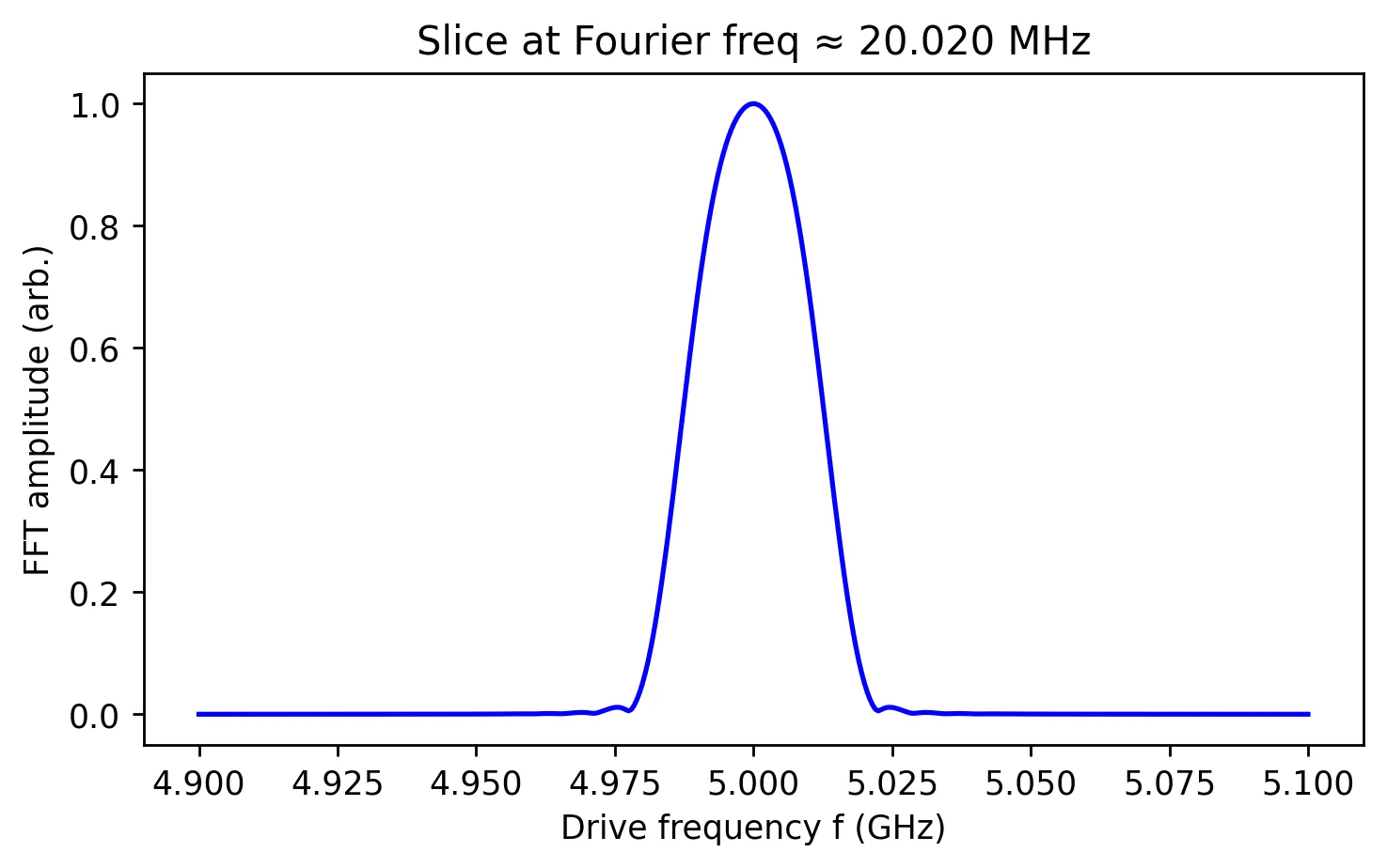
fig.tight_layout(); plt.show()
Run it yourself
More expert notes
Browse all expert notes
Stay in the loop.
Get the latest tutorials, demos, and project showcases straight to your inbox. No noise, just the good stuff.
- 1About the author
- 2Nomenclature and Definitions
- 3Physical Model
- 4Mathematical Foundation
- 5Rotating-Frame Hamiltonian
- 6Excited-State Probability
- 7Phenomenological Dephasing
- 8Detuning and Generalized Rabi Frequency
- 9Quantum Information Interpretation
- 10Bloch-Sphere Interpretation
- 11Fourier Analysis Dynamics
- 12Computational Methodology
- 13Graphical Interpretation
- 14Primary Modeling Assumptions
- 15Notebook Control Knobs
- 16Run it yourself