Pulse Shapes and Envelopes, Visualized
How microwave pulses are shaped to control a quantum chip: Gaussian and sinusoidal envelopes, and the modulated pulses behind common gates.
About the author
Republished with the author's permission from the original notebook. The text, code, and figures below are Onri's, as published.
This notebook authored by Onri Jay Benally shows some plots to help visualize the process of how pulses are shaped to control a quantum chip.
- While Gaussian is prevalent due to its favorable spectral properties, sinusoidal or other shaped envelopes also exist and are actively used in various quantum computing architectures.
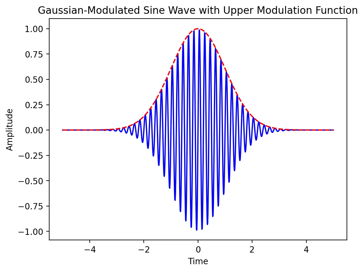
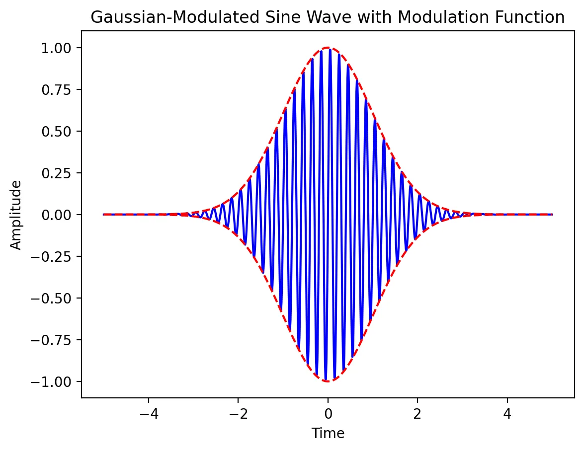
- The choice of modulation function, which resembles an envelope, is dictated by the need to balance gate fidelity, spectral leakage, robustness against noise, and suppression of higher energy transitions.
- Optimal control techniques, such as GRAPE or CRAB, can generate tailored pulse shapes that might include sinusoidal modulations.
- Gradient Ascent Pulse Engineering (GRAPE): A numerical algorithm used in quantum optimal control. It uses time discretization in order to identify the optimal control pulses for quantum systems.
- Chopped Random Basis (CRAB): A method for quantum optimal control that uses a randomly truncated basis to optimize control pulses.
- Derivative Removal by Adiabatic Gate (DRAG): Widely used in implementations of high-fidelity single-qubit gates in superconducting qubit architectures, such as those found in IBM Quantum and Google Quantum processors.
import numpy as np
import matplotlib.pyplot as plt

# Onri prefers using rcParams to increase the quality of all plots to be higher than the default settings.
# This only needs to be done once at beginning of every Jupyter Notebook.
plt.rcParams['figure.dpi'] = 200

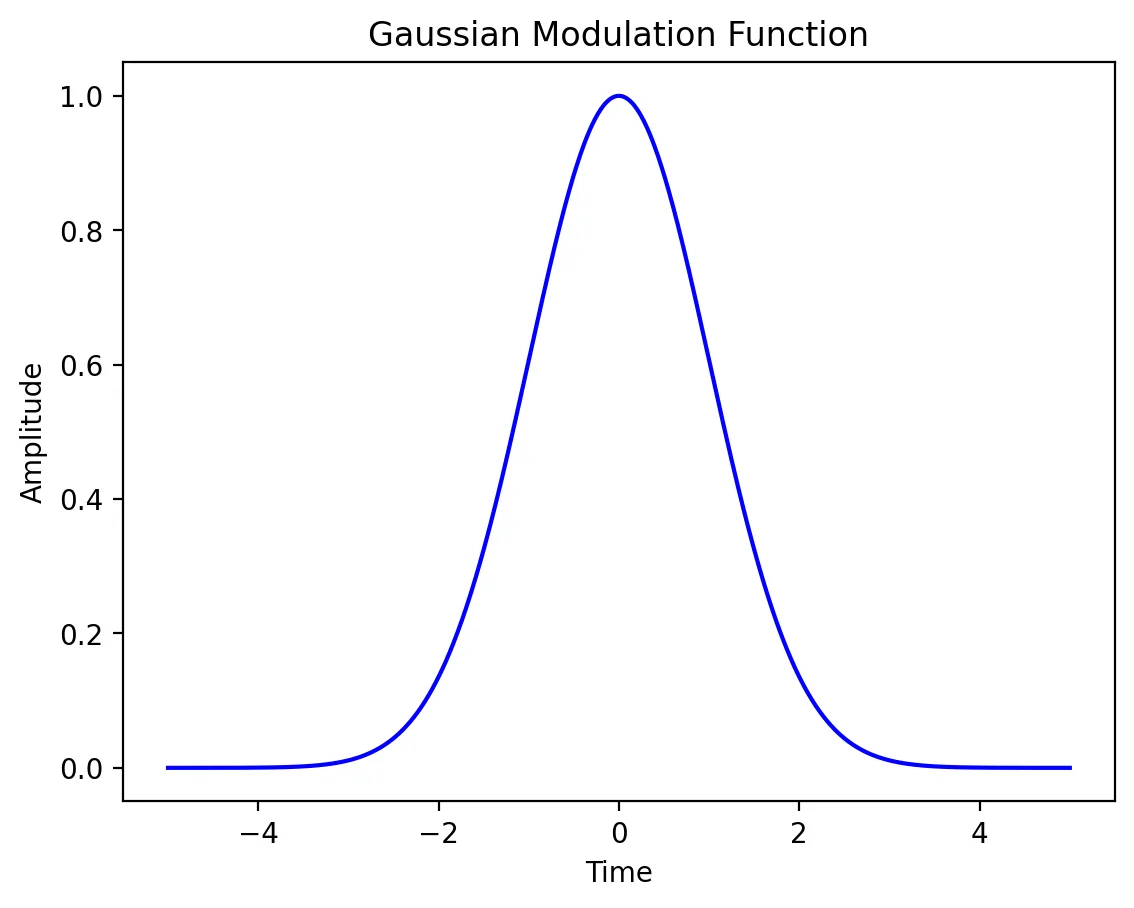
# Define the parameters for the Gaussian modulation function
mean = 0
std_dev = 1
time = np.linspace(-5, 5, 1000)  # Generate time values from -5 to 5

# Calculate the Gaussian modulation function
gaussian_modulation = np.exp(-(time - mean) ** 2 / (2 * std_dev ** 2))

# Plot the Gaussian modulation function with blue color
plt.plot(time, gaussian_modulation, color='blue')
plt.title('Gaussian Modulation Function')
plt.xlabel('Time')
plt.ylabel('Amplitude')
plt.grid(False)
plt.show()
import numpy as np
import matplotlib.pyplot as plt

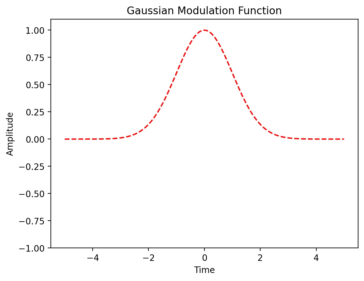
# Define the parameters for the Gaussian modulation function
amplitude = 1
mean = 0
std_dev = 1
time = np.linspace(-5, 5, 1000)  # Generate time values from -5 to 5

# Calculate the Gaussian modulation function
gaussian_modulation = amplitude * np.exp(-(time - mean) ** 2 / (2 * std_dev ** 2))

# Plot the Gaussian modulation function
plt.plot(time, gaussian_modulation, color='red', linestyle='dashed', label='Gaussian Modulation')
plt.title('Gaussian Modulation Function')
plt.xlabel('Time')
plt.ylabel('Amplitude')
plt.ylim(-1.0, 1.1)  # Force the y-axis to display the range from -1.0 to 1.0
# plt.legend()
plt.grid(False)
plt.show()
import numpy as np
import matplotlib.pyplot as plt

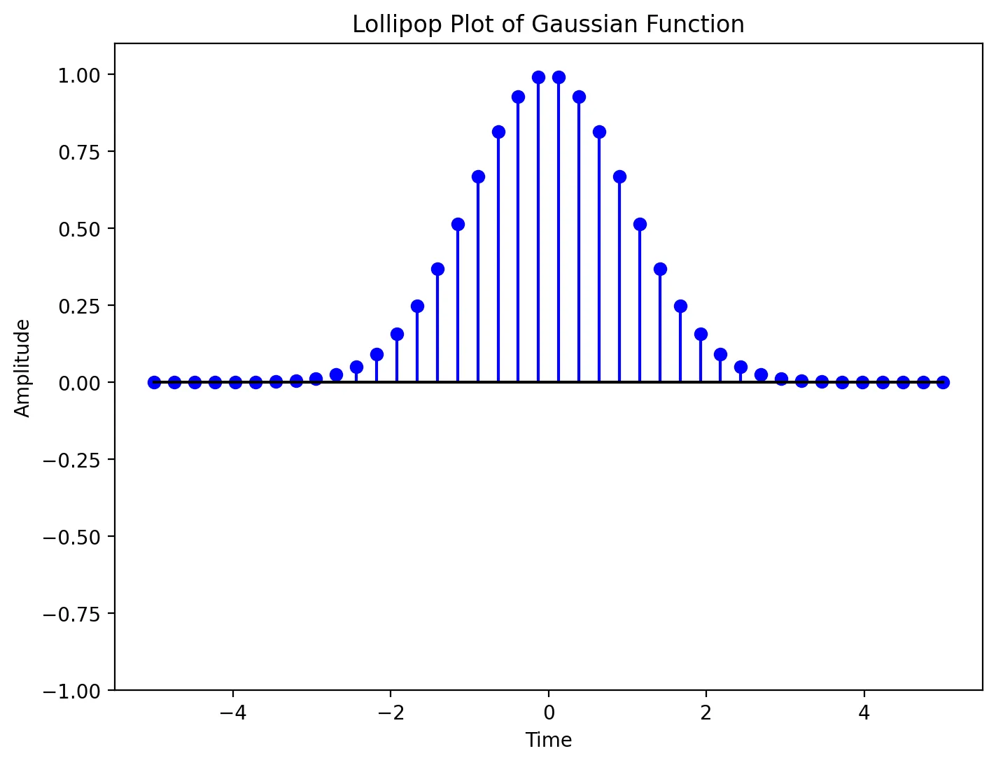
# Define the parameters for the Gaussian function
amplitude = 1
mean = 0
std_dev = 1
time = np.linspace(-5, 5, 20)  # Reduce points for lollipop plot clarity

# Increase the number of points for the lollipop plot
time = np.linspace(-5, 5, 40)  # Doubling the number of points

# Calculate the Gaussian function
gaussian_modulation = amplitude * np.exp(-(time - mean) ** 2 / (2 * std_dev ** 2))

# Create the updated lollipop plot with blue color
plt.figure(figsize=(8, 6))
plt.stem(time, gaussian_modulation, linefmt='b-', markerfmt='bo', basefmt='k-')
plt.title('Lollipop Plot of Gaussian Function')
plt.xlabel('Time')
plt.ylabel('Amplitude')
plt.ylim(-1.0, 1.1)  # Force the y-axis to display the range from -1.0 to 1.1
plt.grid(False)
plt.show()
import numpy as np
import matplotlib.pyplot as plt

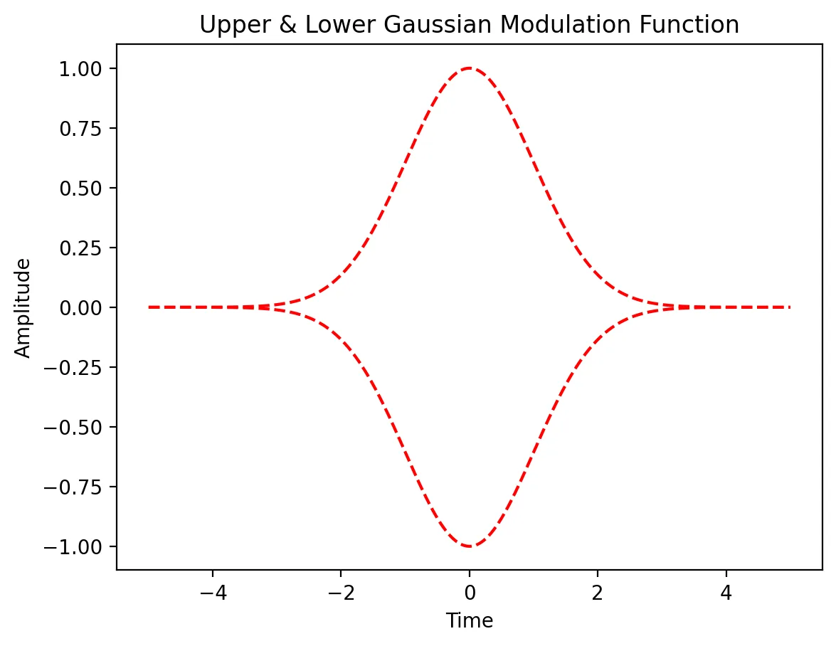
# Define the parameters for the Gaussian-modulated sine wave
amplitude = 1
mean = 0
std_dev = 1
frequency = 5  # Frequency of the sine wave
time = np.linspace(-5, 5, 1000)  # Generate time values from -5 to 5

# Calculate the Gaussian function
gaussian_modulation = np.exp(-(time - mean) ** 2 / (2 * std_dev ** 2))

# Calculate the sine wave
sine_wave = amplitude * np.sin(2 * np.pi * frequency * time)

# Modulate the sine wave with the Gaussian function
gaussian_modulated_sine_wave = gaussian_modulation * sine_wave

# Plot only the function of the Gaussian-modulated sine wave
plt.plot(time, gaussian_modulation, color='red', linestyle='dashed', label='Modulation')
plt.plot(time, -gaussian_modulation, color='red', linestyle='dashed')  # Add the negative function for completeness
plt.title('Upper & Lower Gaussian Modulation Function')
plt.xlabel('Time')
plt.ylabel('Amplitude')
# plt.legend()
plt.grid(False)
plt.show()
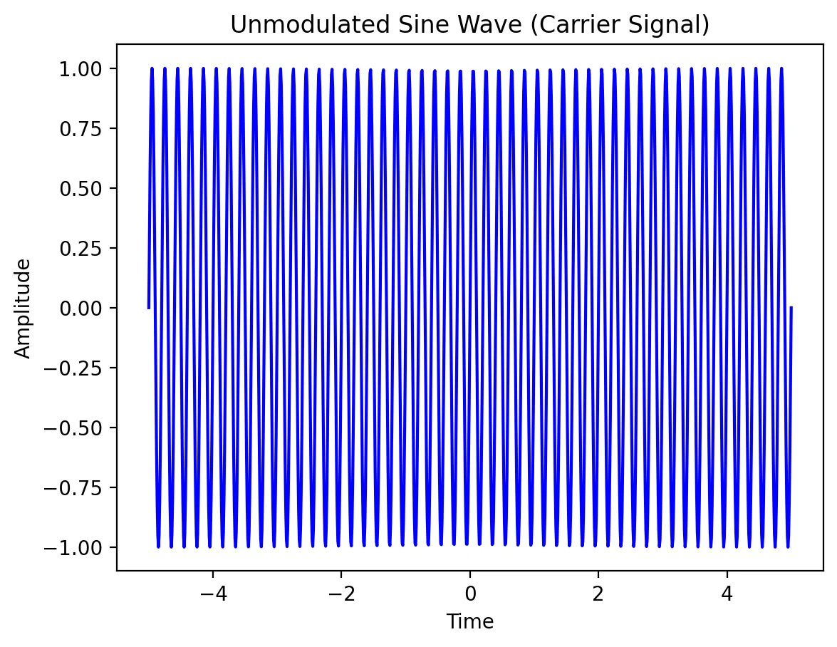
'''
This plot represents a sine wave at a chosen frequency, commonly used to match the resonance frequency
of a quantum device on a chip. In quantum computing, such signals serve as carrier waves for qubit
control pulses before modulation is applied.
'''

import numpy as np
import matplotlib.pyplot as plt

# Define sine wave parameters
amplitude = 1  # Peak amplitude of the wave
frequency = 5  # Frequency of the sine wave (in arbitrary units, could be GHz for quantum systems)
time = np.linspace(-5, 5, 1000)  # Generate 1000 evenly spaced time values from -5 to 5

# Compute the sine wave, representing an unmodulated carrier signal
sine_wave = amplitude * np.sin(2 * np.pi * frequency * time)

# Plot the sine wave with blue color
plt.plot(time, sine_wave, color='blue')
plt.title('Unmodulated Sine Wave (Carrier Signal)')
plt.xlabel('Time')
plt.ylabel('Amplitude')
plt.grid(False)  # No grid for a cleaner look
plt.show()
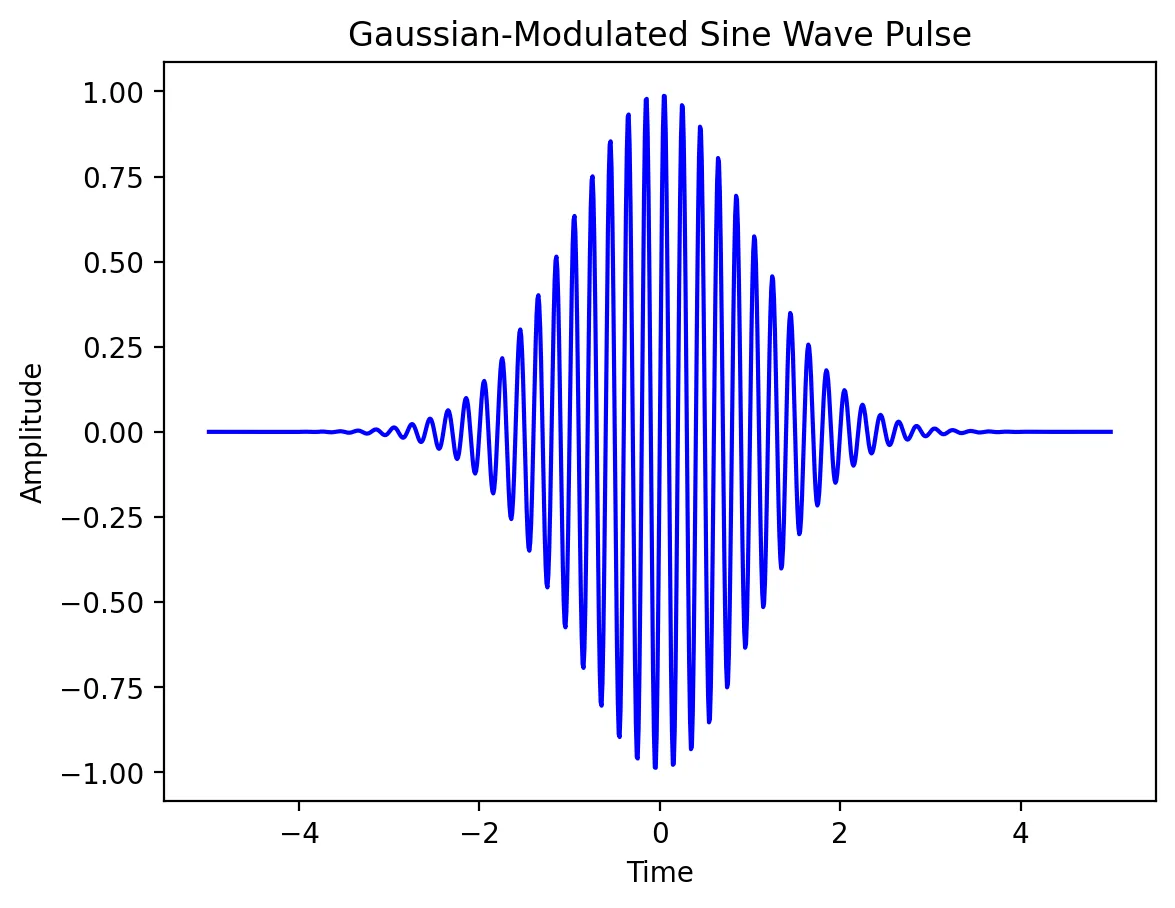
'''
When a modulating pulse shape is applied to an unmodulated sine wave tone, then the result will be a
modulated sine wave output as shown in the plot below. The example shown is modulation by a
Gaussian wave.
'''
import numpy as np
import matplotlib.pyplot as plt

# Define the parameters for the Gaussian-modulated sine wave
amplitude = 1
mean = 0
std_dev = 1
frequency = 5  # Frequency of the sine wave
time = np.linspace(-5, 5, 1000)  # Generate time values from -5 to 5

# Calculate the Gaussian function
gaussian_modulation = np.exp(-(time - mean) ** 2 / (2 * std_dev ** 2))

# Calculate the sine wave
sine_wave = amplitude * np.sin(2 * np.pi * frequency * time)

# Modulate the sine wave with the Gaussian function
gaussian_modulated_sine_wave = gaussian_modulation * sine_wave

# Plot the Gaussian-modulated sine wave with blue color
plt.plot(time, gaussian_modulated_sine_wave, color='blue')
plt.title('Gaussian-Modulated Sine Wave Pulse')
plt.xlabel('Time')
plt.ylabel('Amplitude')
plt.grid(False)
plt.show()
import numpy as np
import matplotlib.pyplot as plt

# Define the parameters for the Gaussian-modulated sine wave
amplitude = 1
mean = 0
std_dev = 1
frequency = 5  # Frequency of the sine wave
time = np.linspace(-5, 5, 1000)  # Generate time values from -5 to 5

# Calculate the Gaussian function
gaussian_modulation = np.exp(-(time - mean) ** 2 / (2 * std_dev ** 2))

# Calculate the sine wave
sine_wave = amplitude * np.sin(2 * np.pi * frequency * time)

# Modulate the sine wave with the Gaussian function
gaussian_modulated_sine_wave = gaussian_modulation * sine_wave

# Calculate the upper envelope of the modulated sine wave
upper_modulation = np.abs(gaussian_modulation)

# Plot the Gaussian-modulated sine wave and its upper envelope
plt.plot(time, gaussian_modulated_sine_wave, color='blue', label='Gaussian-Modulated Sine Wave Pulse')
plt.plot(time, upper_modulation, color='red', linestyle='dashed', label='Upper Modulation Function')
plt.title('Gaussian-Modulated Sine Wave with Upper Modulation Function')
plt.xlabel('Time')
plt.ylabel('Amplitude')
# plt.legend()
plt.grid(False)
plt.show()
import numpy as np
import matplotlib.pyplot as plt

# Define the parameters for the Gaussian-modulated sine wave
amplitude = 1
mean = 0
std_dev = 1
frequency = 5  # Frequency of the sine wave
time = np.linspace(-5, 5, 1000)  # Generate time values from -5 to 5

# Calculate the Gaussian function
gaussian_modulation = np.exp(-(time - mean) ** 2 / (2 * std_dev ** 2))

# Calculate the sine wave
sine_wave = amplitude * np.sin(2 * np.pi * frequency * time)

# Modulate the sine wave with the Gaussian function
gaussian_modulated_sine_wave = gaussian_modulation * sine_wave

# Calculate the function of the modulated sine wave
modulation = np.abs(gaussian_modulation)

# Plot the Gaussian-modulated sine wave and its modulation function
plt.plot(time, gaussian_modulated_sine_wave, color='blue', label='Gaussian-Modulated Sine Wave Pulse')
plt.plot(time, modulation, color='red', linestyle='dashed', label='Modulation')
plt.plot(time, -modulation, color='red', linestyle='dashed')  # Add the negative modulation function for completeness
plt.title('Gaussian-Modulated Sine Wave with Modulation Function')
plt.xlabel('Time')
plt.ylabel('Amplitude')
# plt.legend()
plt.grid(False)
plt.show()
Below are some common pulse envelope shapes used to modulate a sine wave tone.
import numpy as np
import matplotlib.pyplot as plt
from scipy.signal.windows import blackmanharris, tukey

# Define time vector
t = np.linspace(-2, 2, 1000)

# Define different pulse envelopes
gaussian = np.exp(-t**2)
sin2 = np.sin(np.pi * (t - t.min()) / (t.max() - t.min()))**2
cos2 = np.cos(np.pi * (t - t.min()) / (t.max() - t.min()))**2
rectangular = np.ones_like(t)
rectangular[np.abs(t) > 1] = 0
blackman_harris = blackmanharris(len(t))
tukey_envelope = tukey(len(t), alpha=0.5)
sech = 1 / np.cosh(t)

# List of envelopes and titles
envelopes = [(gaussian, "Gaussian Modulation Function"),
             (sin2, "$Sin^{2}$ Modulation Function"),
             (cos2, "$Cos^{2}$ Modulation Function"),
             (rectangular, "Rectangular Modulation Function"),
             (blackman_harris, "Blackman-Harris Modulation Function"),
             (tukey_envelope, "Tukey Modulation Function"),
             (sech, "Sech Modulation Function")]

# Create subplots
fig, axes = plt.subplots(3, 3, figsize=(12, 9))
axes = axes.flatten()

for i, (envelope, title) in enumerate(envelopes):
    axes[i].plot(t, envelope, 'b')
    axes[i].set_title(title)
    axes[i].set_xlabel("Time")
    axes[i].set_ylabel("Amplitude")
    # axes[i].legend([title])

# Hide unused subplots
for j in range(i + 1, len(axes)):
    fig.delaxes(axes[j])

plt.tight_layout()
plt.show()
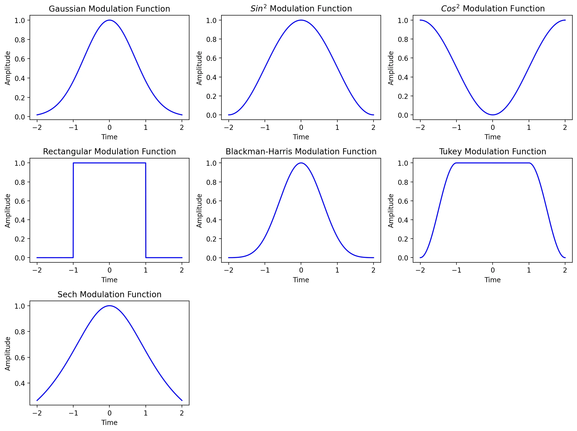
import numpy as np
import matplotlib.pyplot as plt
from scipy.signal.windows import blackmanharris, tukey

# Define time vector with reduced points for lollipop plot clarity
t = np.linspace(-2, 2, 40)

# Define different modulation functions
gaussian_modulation = np.exp(-t**2)
sin2_modulation = np.sin(np.pi * (t - t.min()) / (t.max() - t.min()))**2
cos2_modulation = np.cos(np.pi * (t - t.min()) / (t.max() - t.min()))**2
rectangular_modulation = np.ones_like(t)
rectangular_modulation[np.abs(t) > 1] = 0
blackman_harris_modulation = blackmanharris(len(t))
tukey_modulation = tukey(len(t), alpha=0.5)
sech_modulation = 1 / np.cosh(t)

# List of modulation functions and titles
modulations = [(gaussian_modulation, "Gaussian Modulation Function"),
               (sin2_modulation, "Sin² Modulation Function"),
               (cos2_modulation, "Cos² Modulation Function"),
               (rectangular_modulation, "Rectangular Modulation Function"),
               (blackman_harris_modulation, "Blackman-Harris Modulation Function"),
               (tukey_modulation, "Tukey Modulation Function"),
               (sech_modulation, "Sech Modulation Function")]

# Create subplots
fig, axes = plt.subplots(3, 3, figsize=(12, 9))
axes = axes.flatten()

for i, (modulation, title) in enumerate(modulations):
    axes[i].stem(t, modulation, linefmt='b-', markerfmt='bo', basefmt='k-')
    axes[i].set_title(title)
    axes[i].set_xlabel("Time")
    axes[i].set_ylabel("Amplitude")

# Hide unused subplots
for j in range(i + 1, len(axes)):
    fig.delaxes(axes[j])

plt.tight_layout()
plt.show()
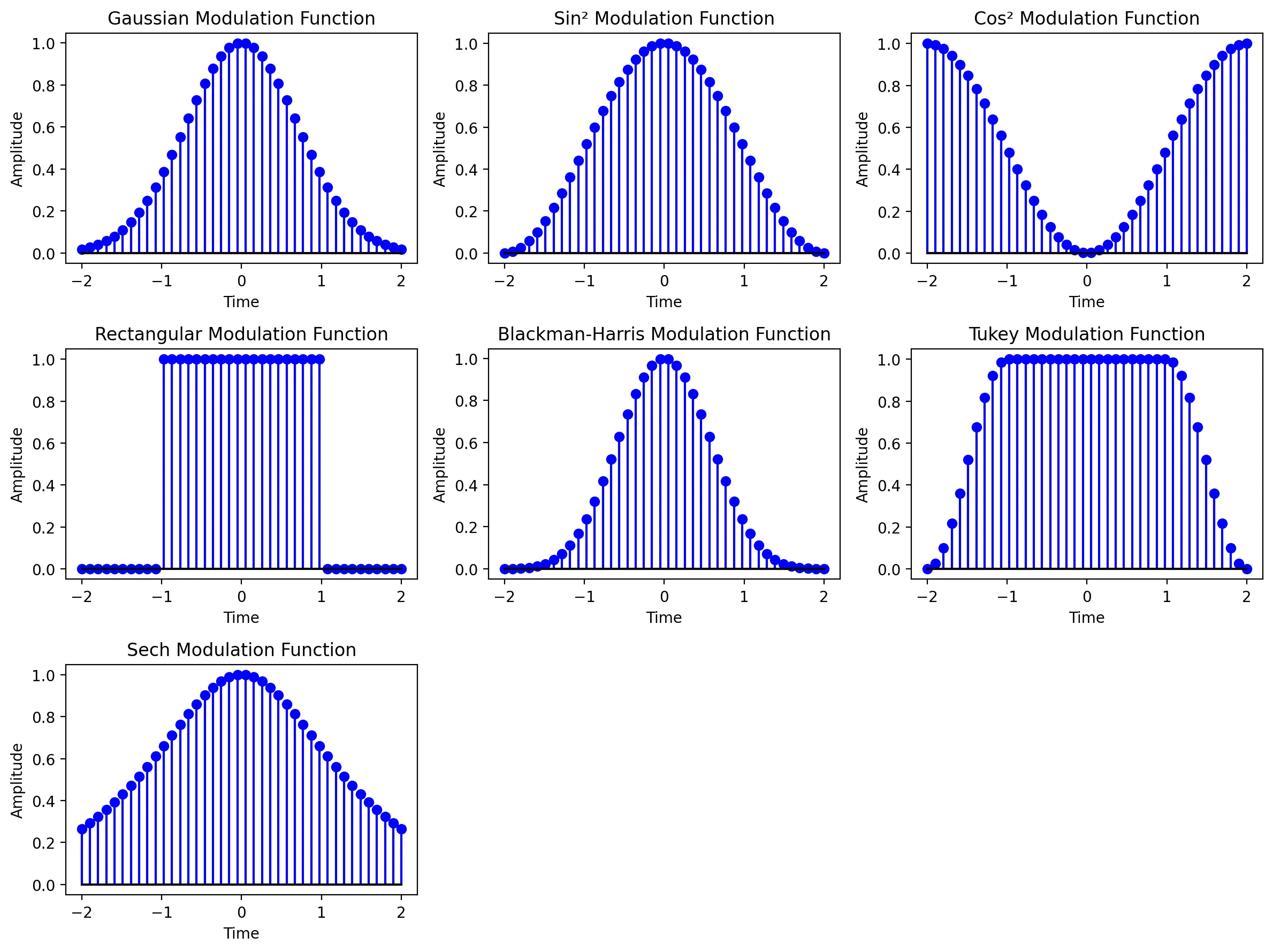
import numpy as np
import matplotlib.pyplot as plt
from scipy.signal.windows import blackmanharris, tukey

# Define time vector
time = np.linspace(-5, 5, 1000)

# Define different modulated sine waves
gaussian_modulated_sine = np.exp(-time**2)
sin2_modulated_sine = np.sin(np.pi * (time - time.min()) / (time.max() - time.min()))**2
cos2_modulated_sine = np.cos(np.pi * (time - time.min()) / (time.max() - time.min()))**2
rectangular_modulated_sine = np.ones_like(time)
rectangular_modulated_sine[np.abs(time) > 2] = 0
blackman_harris_modulated_sine = blackmanharris(len(time))
tukey_modulated_sine = tukey(len(time), alpha=0.5)
sech_modulated_sine = 1 / np.cosh(time)

# Define sine wave parameters
amplitude = 1
frequency = 5  # Frequency of the sine wave
sine_wave = amplitude * np.sin(2 * np.pi * frequency * time)

# List of modulated sine waves and titles
modulated_sines = [(gaussian_modulated_sine, "Gaussian Modulated Sine Wave"),
                    (sin2_modulated_sine, "$Sin^{2}$ Modulated Sine Wave"),
                    (cos2_modulated_sine, "$Cos^{2}$ Modulated Sine Wave"),
                    (rectangular_modulated_sine, "Rectangular Modulated Sine Wave"),
                    (blackman_harris_modulated_sine, "Blackman-Harris Modulated Sine Wave"),
                    (tukey_modulated_sine, "Tukey Modulated Sine Wave"),
                    (sech_modulated_sine, "Sech Modulated Sine Wave")]

# Create subplots
fig, axes = plt.subplots(3, 3, figsize=(12, 9))
axes = axes.flatten()

for i, (modulated_sine, title) in enumerate(modulated_sines):
    modulated_wave = modulated_sine * sine_wave
    axes[i].plot(time, modulated_wave, 'b')
    axes[i].set_title(title)
    axes[i].set_xlabel("Time")
    axes[i].set_ylabel("Amplitude")

# Hide unused subplots
for j in range(i + 1, len(axes)):
    fig.delaxes(axes[j])

plt.tight_layout()
plt.show()
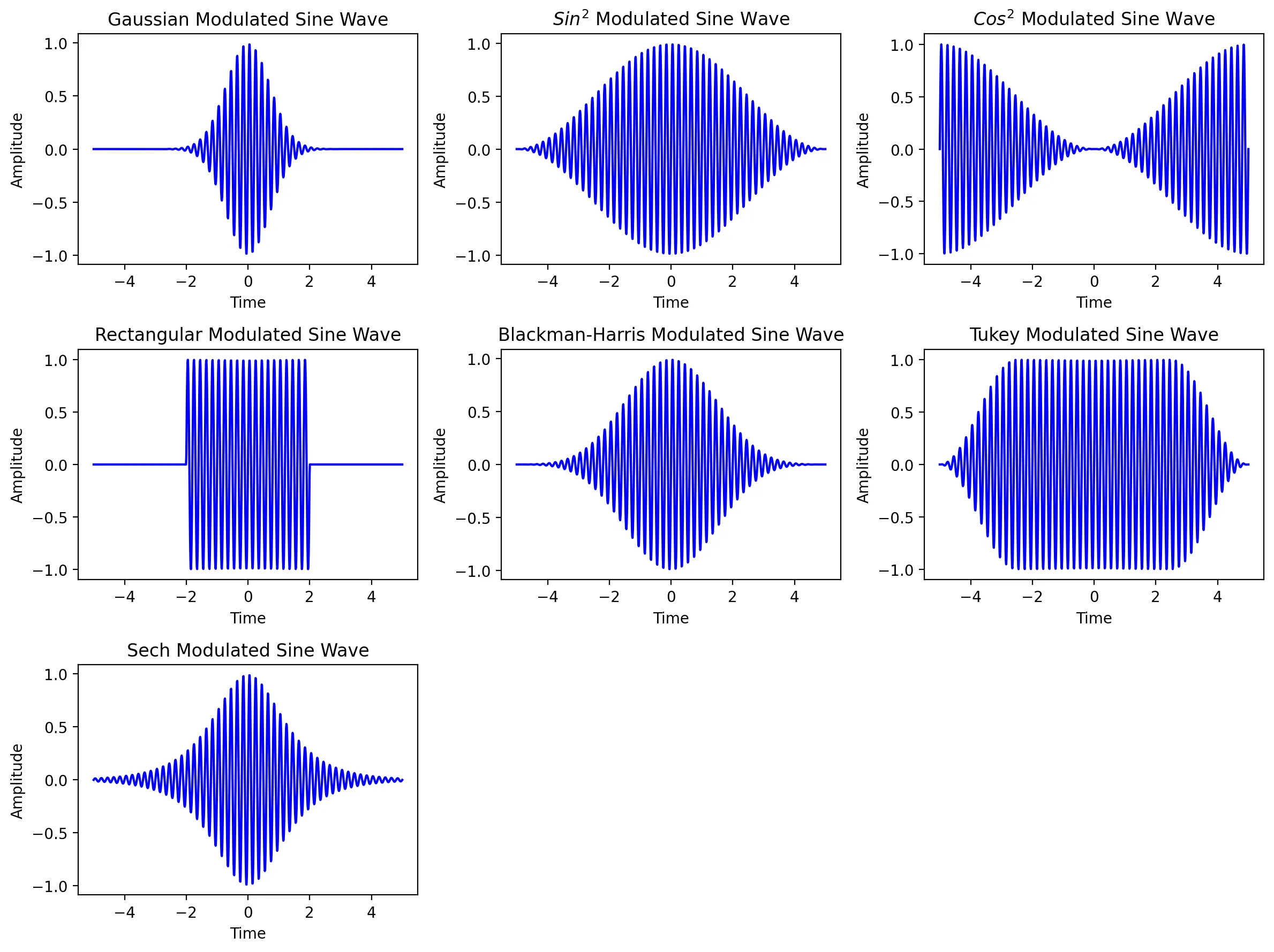
import numpy as np
import matplotlib.pyplot as plt
from scipy.signal.windows import blackmanharris, tukey

# Define time vector
time = np.linspace(-5, 5, 1000)

# Define different modulated sine waves
gaussian_modulated_sine = np.exp(-time**2)
sin2_modulated_sine = np.sin(np.pi * (time - time.min()) / (time.max() - time.min()))**2
cos2_modulated_sine = np.cos(np.pi * (time - time.min()) / (time.max() - time.min()))**2
rectangular_modulated_sine = np.ones_like(time)
rectangular_modulated_sine[np.abs(time) > 2] = 0
blackman_harris_modulated_sine = blackmanharris(len(time))
tukey_modulated_sine = tukey(len(time), alpha=0.5)
sech_modulated_sine = 1 / np.cosh(time)

# Define sine wave parameters
amplitude = 1
frequency = 5  # Frequency of the sine wave
sine_wave = amplitude * np.sin(2 * np.pi * frequency * time)

# List of modulated sine waves and titles
modulated_sines = [(gaussian_modulated_sine, "Gaussian Modulated Sine Wave"),
                   (sin2_modulated_sine, "$Sin^{2}$ Modulated Sine Wave"),
                   (cos2_modulated_sine, "$Cos^{2}$ Modulated Sine Wave"),
                   (rectangular_modulated_sine, "Rectangular Modulated Sine Wave"),
                   (blackman_harris_modulated_sine, "Blackman-Harris Modulated Sine Wave"),
                   (tukey_modulated_sine, "Tukey Modulated Sine Wave"),
                   (sech_modulated_sine, "Sech Modulated Sine Wave")]

# Create subplots
fig, axes = plt.subplots(3, 3, figsize=(12, 9))
axes = axes.flatten()

for i, (modulated_sine, title) in enumerate(modulated_sines):
    modulated_wave = modulated_sine * sine_wave
    axes[i].plot(time, modulated_wave, 'b')
    axes[i].plot(time, modulated_sine, 'r', linestyle='--', label='Upper Modulation Function')
    axes[i].set_title(title)
    axes[i].set_xlabel("Time")
    axes[i].set_ylabel("Amplitude")
    axes[i].legend()

# Hide unused subplots
for j in range(i + 1, len(axes)):
    fig.delaxes(axes[j])

plt.tight_layout()
plt.show()
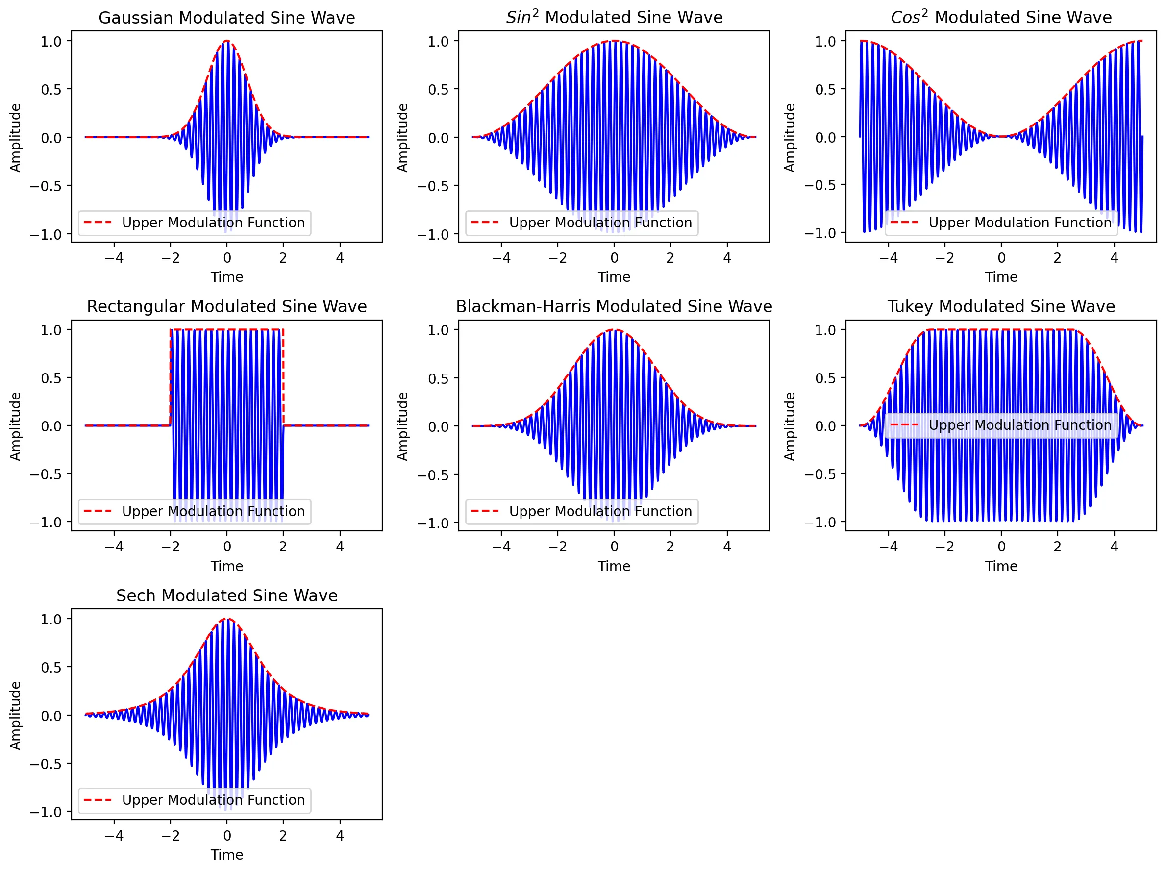
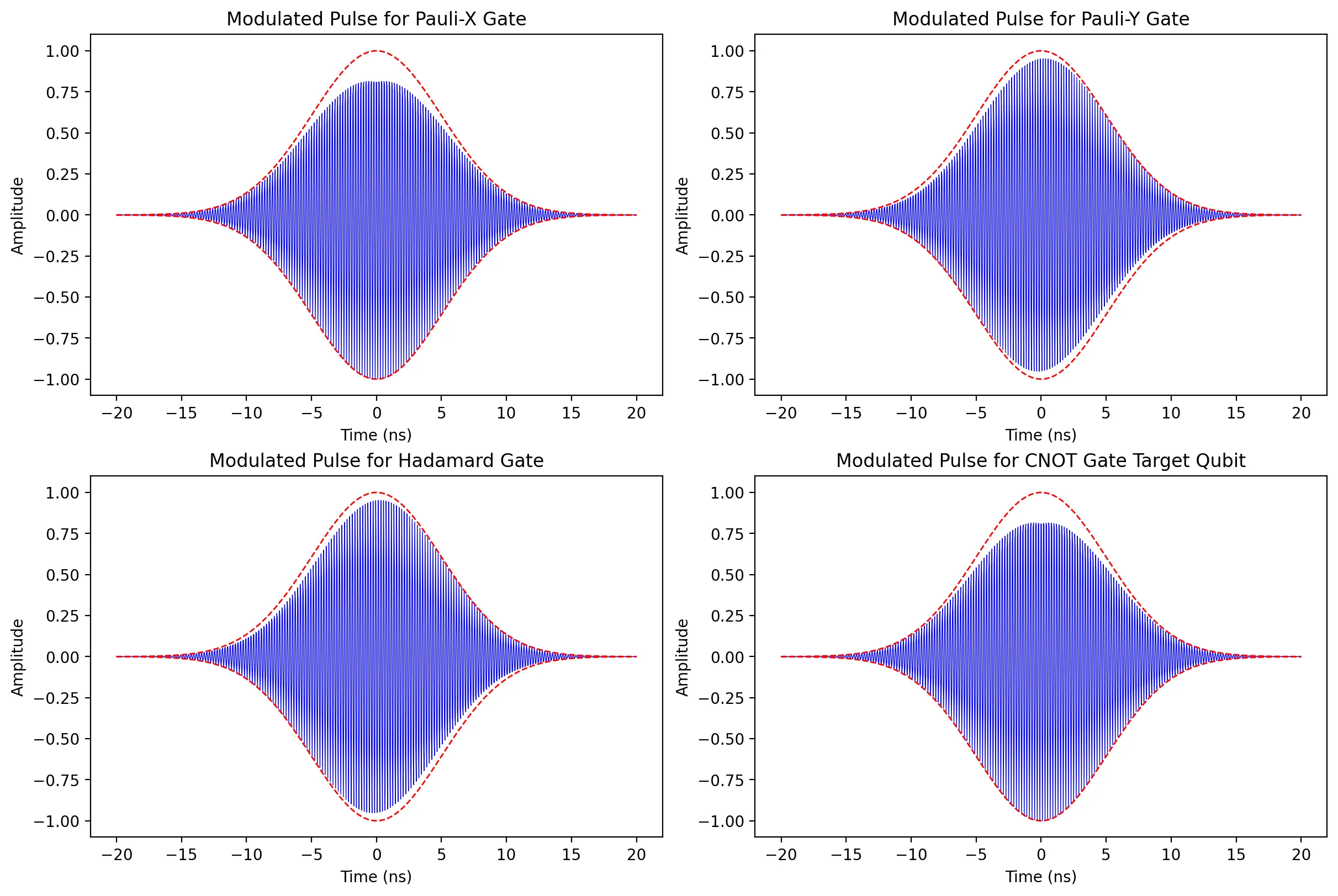
Below are some applied examples in the context of common quantum gates.
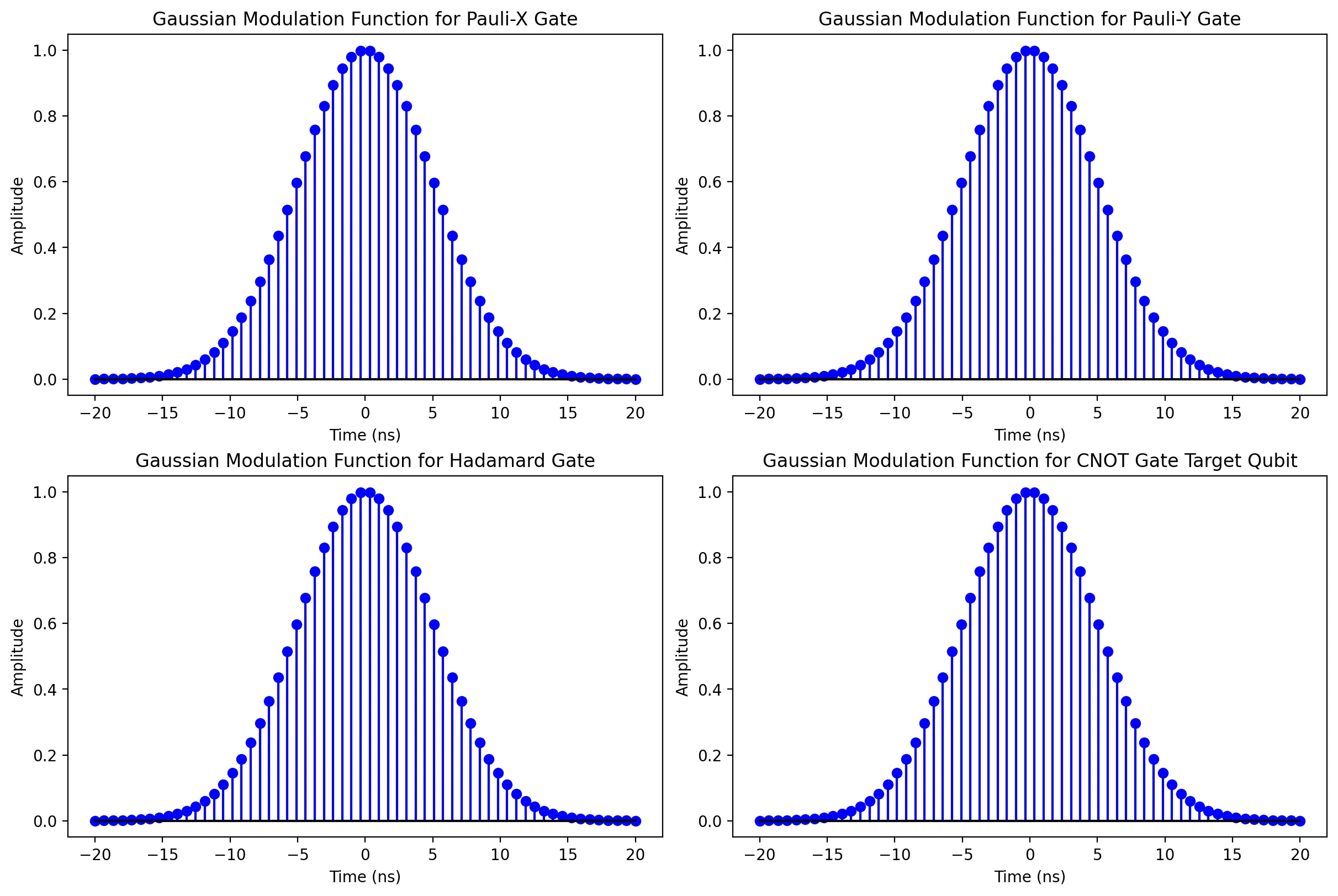
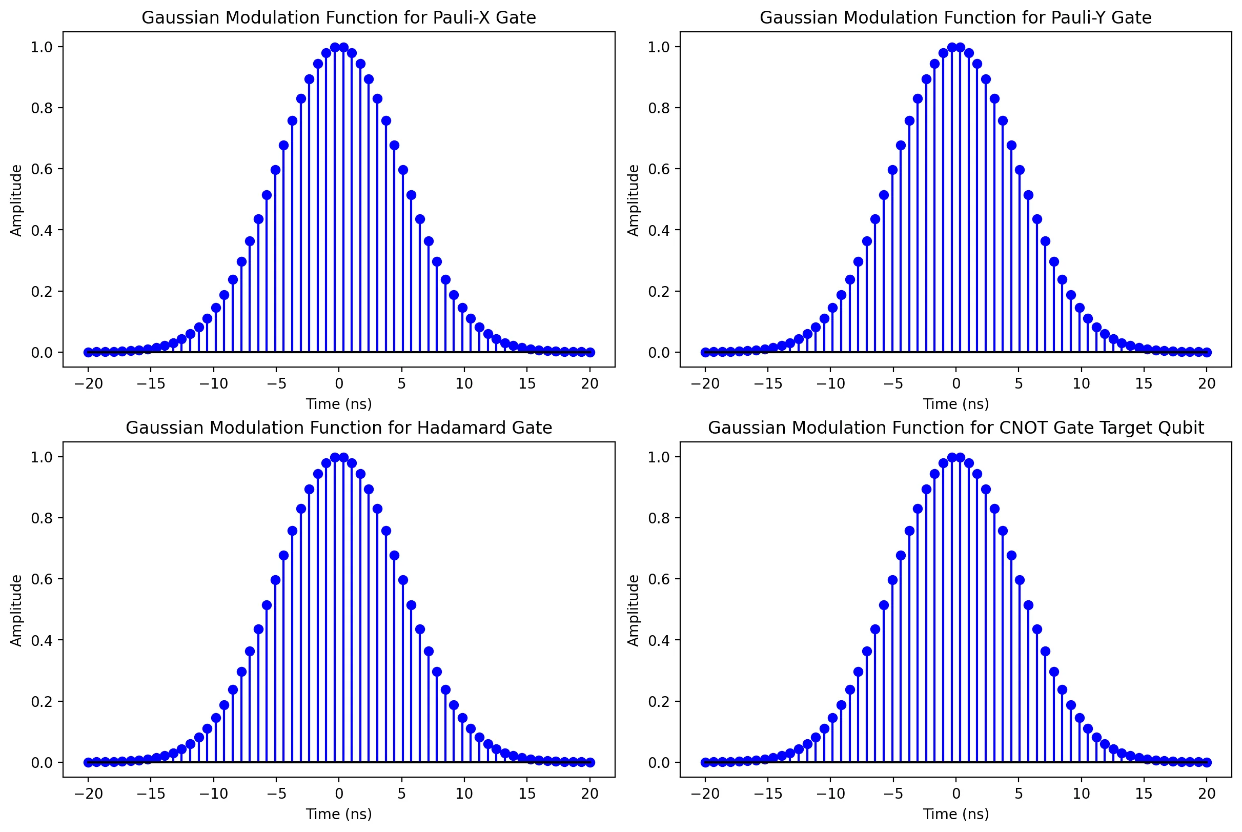
Relevant equations for the modulated Gaussian pulses used in the plots for some common quantum gates:
1. Gaussian Envelope
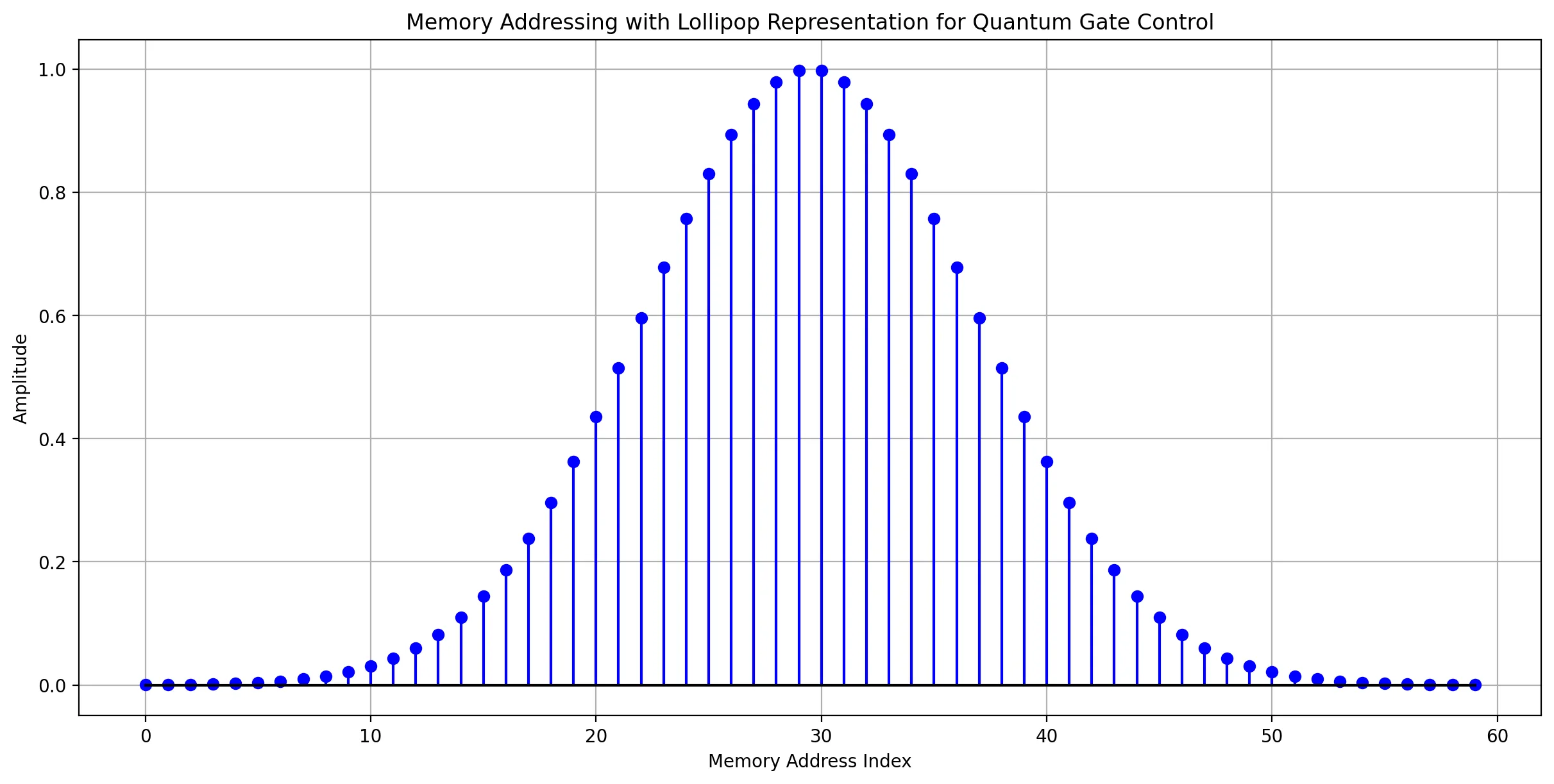
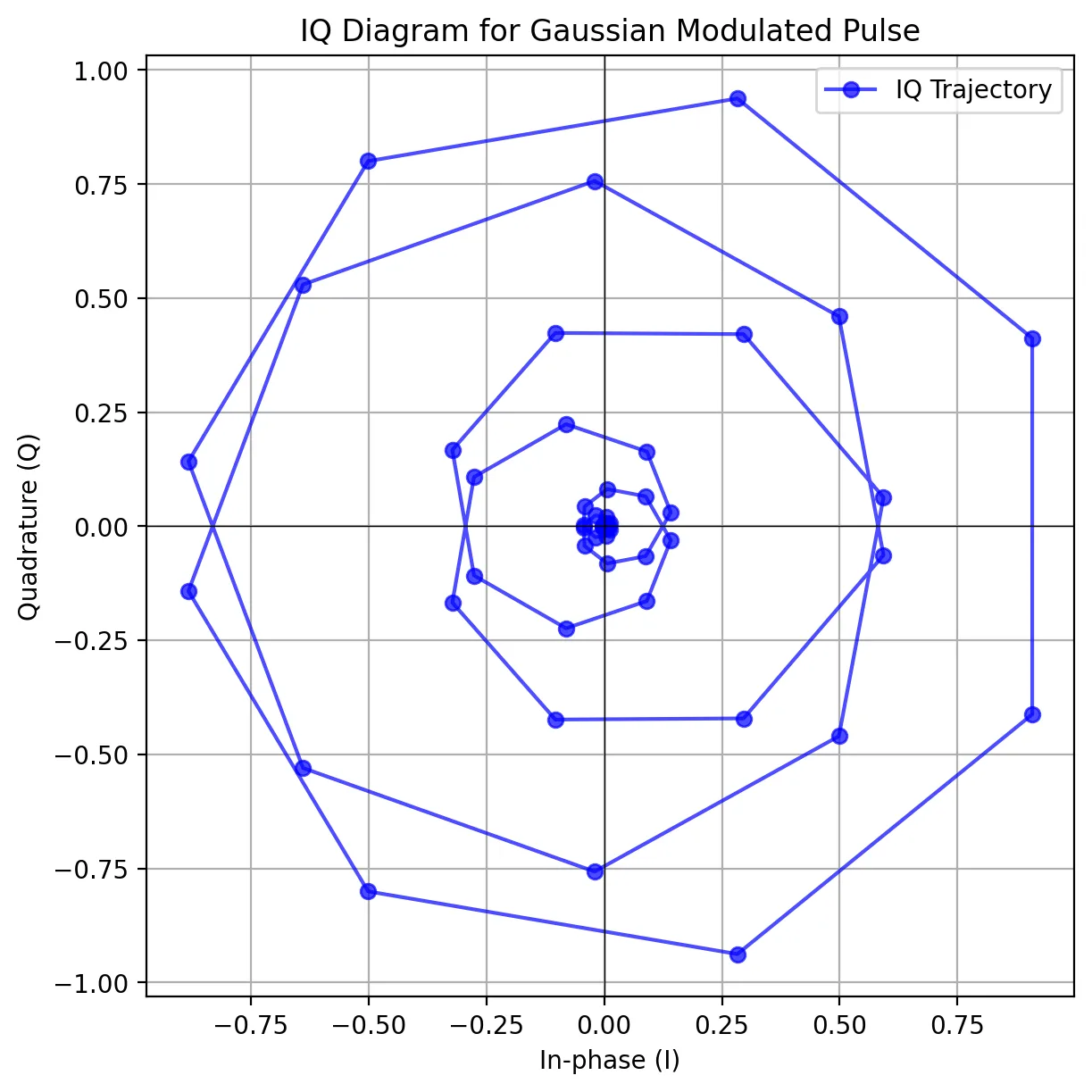
The Gaussian envelope is used to smoothly shape the pulse to minimize spectral leakage: where:
- is the peak amplitude,
- is the pulse center,
- determines the width of the pulse.
2. Modulated Pulse for Pauli-X Gate
The Pauli-X gate is implemented with a zero-phase cosine modulation: where:
- is the carrier frequency (typically GHz range),
- for an X gate.
- The modulation is centered at the qubit frequency with zero phase shift, leading to a cosine-like oscillation.
3. Modulated Pulse for Pauli-Y Gate
The Pauli-Y gate is implemented with a phase-shifted cosine modulation: where:
- shifts the phase by 90° (producing a sine-like waveform).
- The modulation has a phase shift, which shifts the waveform by a quarter cycle, making it a sine-like oscillation.
4. Why No Pulse for Pauli-Z Gate?
For Pauli-Z , no physical pulse is needed because it is implemented as a virtual phase shift: This shift is typically done in software rather than by applying a physical pulse.
Relevant equations in table form, for the modulated Gaussian pulses used in the plots for some common quantum gates:
| Gate | Equation |
|---|---|
| Gaussian Envelope | |
| Pauli-X Gate | |
| Pauli-Y Gate | |
| Hadamard Gate | |
| CNOT Target Qubit Pulse |
import numpy as np
import matplotlib.pyplot as plt

# Define parameters
t0 = 0      # Pulse center
sigma = 5   # Standard deviation of Gaussian modulation function (ns)
A0 = 1      # Peak amplitude

# Increase the number of points by 1.5x for denser lollipop visualization
num_points = int(40 * 1.5)
t = np.linspace(-20, 20, num_points)  # Adjusted time axis

# Compute Gaussian modulation function
gaussian_modulation = A0 * np.exp(-(t - t0)**2 / (2 * sigma**2))

# Store modulation functions and titles in an array
modulations = [
    (gaussian_modulation, "Gaussian Modulation Function for Pauli-X Gate"),
    (gaussian_modulation, "Gaussian Modulation Function for Pauli-Y Gate"),
    (gaussian_modulation, "Gaussian Modulation Function for Hadamard Gate"),
    (gaussian_modulation, "Gaussian Modulation Function for CNOT Gate Target Qubit")
]

# Create a figure with constrained layout
fig, axs = plt.subplots(2, 2, figsize=(12, 8), constrained_layout=True)
axs = axs.flatten()

# Lollipop plot setup
for ax, (modulation, title) in zip(axs, modulations):
    ax.stem(t, modulation, linefmt='b-', markerfmt='bo', basefmt='k-')
    ax.set_title(title)
    ax.set_xlabel("Time (ns)")
    ax.set_ylabel("Amplitude")

# Memory Addressing with Lollipop Representation
fig_combined, ax_combined = plt.subplots(figsize=(12, 6), constrained_layout=True)

# Memory addresses as an index range
memory_addresses = np.arange(len(t))

# Lollipop-style plot for memory addressing
ax_combined.stem(memory_addresses, gaussian_modulation, linefmt='b-', markerfmt='bo', basefmt='k-')

# Labels and title
ax_combined.set_title("Memory Addressing with Lollipop Representation for Quantum Gate Control")
ax_combined.set_xlabel("Memory Address Index")
ax_combined.set_ylabel("Amplitude")
ax_combined.grid(True)

# Display plots
plt.show()
import numpy as np
import matplotlib.pyplot as plt

# Define parameters
t0 = 0      # Pulse center
sigma = 5   # Standard deviation of Gaussian modulation function (ns)
A0 = 1      # Peak amplitude
frequency = 0.2  # Frequency of the carrier wave (normalized)

# Increase the number of points by 1.5x for denser visualization
num_points = int(40 * 1.5)
t = np.linspace(-20, 20, num_points)  # Adjusted time axis

# Compute Gaussian modulation function
gaussian_modulation = A0 * np.exp(-(t - t0)**2 / (2 * sigma**2))

# Generate In-phase (I) and Quadrature (Q) components
I = gaussian_modulation * np.cos(2 * np.pi * frequency * t)
Q = gaussian_modulation * np.sin(2 * np.pi * frequency * t)

# Plot IQ diagram
fig, ax = plt.subplots(figsize=(6, 6), constrained_layout=True)
ax.plot(I, Q, 'bo-', alpha=0.7, label="IQ Trajectory")
ax.set_xlabel("In-phase (I)")
ax.set_ylabel("Quadrature (Q)")
ax.set_title("IQ Diagram for Gaussian Modulated Pulse")
ax.axhline(0, color='k', linewidth=0.5)
ax.axvline(0, color='k', linewidth=0.5)
ax.grid(True)
ax.legend()

plt.show()
import numpy as np
import matplotlib.pyplot as plt

# Define parameters
t0 = 0      # Pulse center
sigma = 5   # Standard deviation of Gaussian modulation function (ns)
A0 = 1      # Peak amplitude

# Increase the number of points by 1.5x for denser lollipop visualization
num_points = int(40 * 1.5)
t = np.linspace(-20, 20, num_points)  # Adjusted time axis

# Compute Gaussian modulation function
gaussian_modulation = A0 * np.exp(-(t - t0)**2 / (2 * sigma**2))

# Store modulation functions and titles in an array
modulations = [
    (gaussian_modulation, "Gaussian Modulation Function for Pauli-X Gate"),
    (gaussian_modulation, "Gaussian Modulation Function for Pauli-Y Gate"),
    (gaussian_modulation, "Gaussian Modulation Function for Hadamard Gate"),
    (gaussian_modulation, "Gaussian Modulation Function for CNOT Gate Target Qubit")
]

# Create lollipop plots
fig, axs = plt.subplots(2, 2, figsize=(12, 8), constrained_layout=True)
axs = axs.flatten()

for ax, (modulation, title) in zip(axs, modulations):
    ax.stem(t, gaussian_modulation, linefmt='b-', markerfmt='bo', basefmt='k-')
    ax.set_title(title)
    ax.set_xlabel("Time (ns)")
    ax.set_ylabel("Amplitude")

plt.show()
import numpy as np
import matplotlib.pyplot as plt

# Define parameters
t0 = 0      # Pulse center
sigma = 5   # Standard deviation of Gaussian modulation (ns)
A0 = 1      # Peak amplitude
fc = 5e9    # Carrier frequency (5 GHz, typical for superconducting qubits)
phi_X = 0           # X gate (Pauli-X) - $\pi$ rotation around X-axis
phi_Y = np.pi / 2   # Y gate (Pauli-Y) - $\pi/2$ rotation around Y-axis
phi_H = np.pi / 2   # Hadamard gate (H) - $\pi/2$ rotation around Y-axis
t = np.linspace(-20, 20, 1000)  # Time axis in nanoseconds

# Compute Gaussian modulation function
gaussian_envelope = A0 * np.exp(-(t - t0)**2 / (2 * sigma**2))

# Compute modulated pulses for X, Y, H, and CNOT gates
modulated_pulse_X = gaussian_envelope * np.cos(2 * np.pi * fc * t * 1e-9 + phi_X)
modulated_pulse_Y = gaussian_envelope * np.cos(2 * np.pi * fc * t * 1e-9 + phi_Y)
modulated_pulse_H = gaussian_envelope * np.cos(2 * np.pi * fc * t * 1e-9 + phi_H)
modulated_pulse_CNOT = gaussian_envelope * np.cos(2 * np.pi * fc * t * 1e-9 + phi_X)  # Similar to X gate

# Store pulses and titles in an array
pulses = np.array([
    (modulated_pulse_X, "Pauli-X Gate"),
    (modulated_pulse_Y, "Pauli-Y Gate"),
    (modulated_pulse_H, "Hadamard Gate"),
    (modulated_pulse_CNOT, "CNOT Gate Target Qubit")
], dtype=object)

# Create plots with blue pulse lines
fig, axs = plt.subplots(2, 2, figsize=(12, 8), constrained_layout=True)
axs = axs.flatten()

for ax, (pulse, title) in zip(axs, pulses):
    ax.plot(t, pulse, 'b', linewidth=0.5, label=f"{title} Modulated Pulse")  # Blue line with reduced thickness
    ax.plot(t, gaussian_envelope, 'r--', linewidth=1.0, label="Gaussian Envelope")
    ax.plot(t, -gaussian_envelope, 'r--', linewidth=1.0)
    ax.set_title(f"Modulated Pulse for {title}")
    ax.set_xlabel("Time (ns)")
    ax.set_ylabel("Amplitude")
    # ax.legend()
    # ax.grid()

plt.show()
More expert notes
Browse all expert notes
Stay in the loop.
Get the latest tutorials, demos, and project showcases straight to your inbox. No noise, just the good stuff.