Deep dive · Hardware
Cross-Resonance Gate: Slices and Heatmaps
How the ZX entangling rate and static ZZ vary with detuning and drive amplitude, plotted from the PRA 2020 cross-resonance formulas.
About the author
Republished with the author's permission from the original notebook and shared under CC-BY-4.0. The text, code, and figures below are Onri's, as published.
Cross-Resonance (CR) Gate
| # | Figure | What to notice |
|---|---|---|
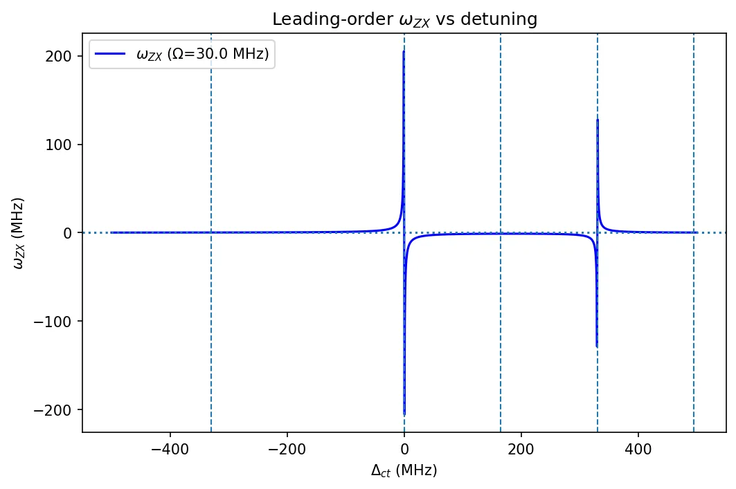
| 1 | vs (slice at fixed ) | Entangling-rate sign flips at poles; magnitude peaks between poles; roughly linear in drive amplitude . |
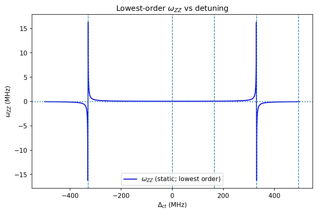
| 2 | vs | Static varies strongly near poles; lowest between poles; independent of at leading order. |
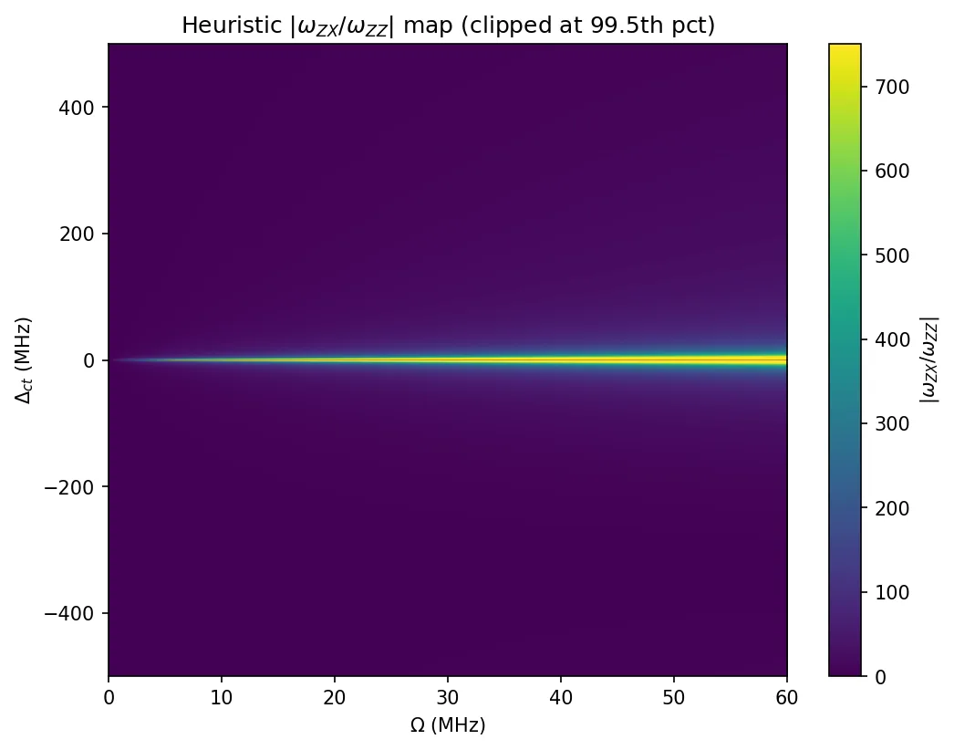
| 3 | vs | Heuristic speed-vs-static figure; tall regions mark friendlier operating points (away from poles). |
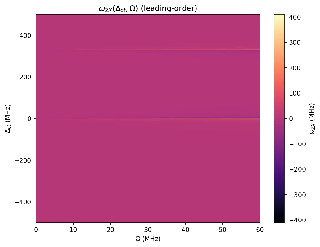
| 4 | heatmap | Linear growth with ; detuning structure set by anharmonicities; region boundaries visible as sharp changes. |
| 5 | heatmap | Bright bands away from poles suggest high entangling-rate with low static (good for echoed-CR). |
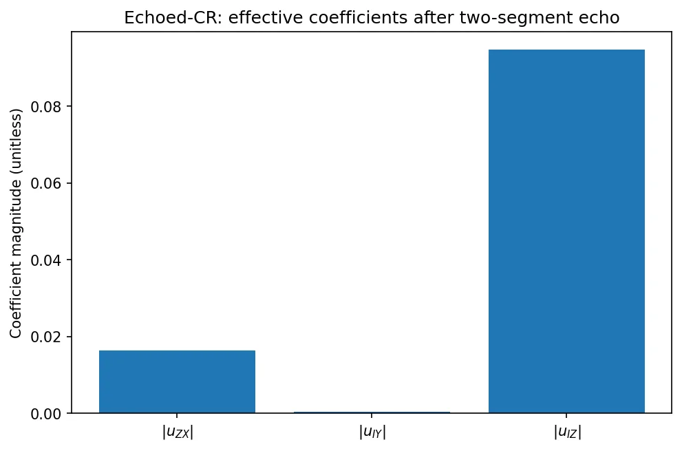
| 6 | Echoed-CR coefficients (two-segment echo) | Echo preserves odd-in- and suppresses even-in- terms (, ) to first order. |
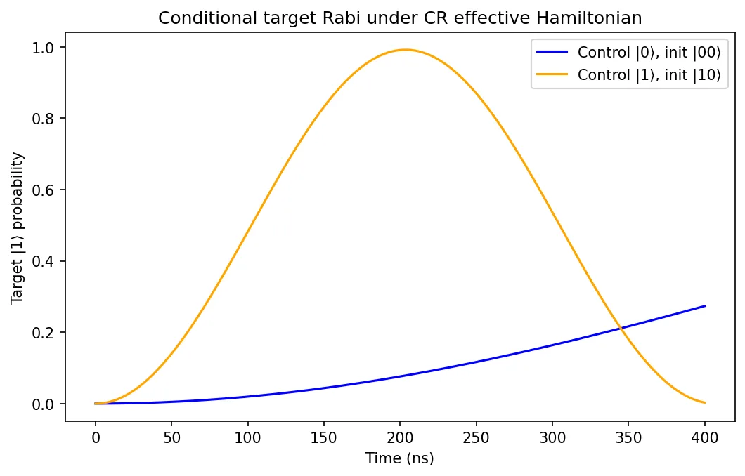
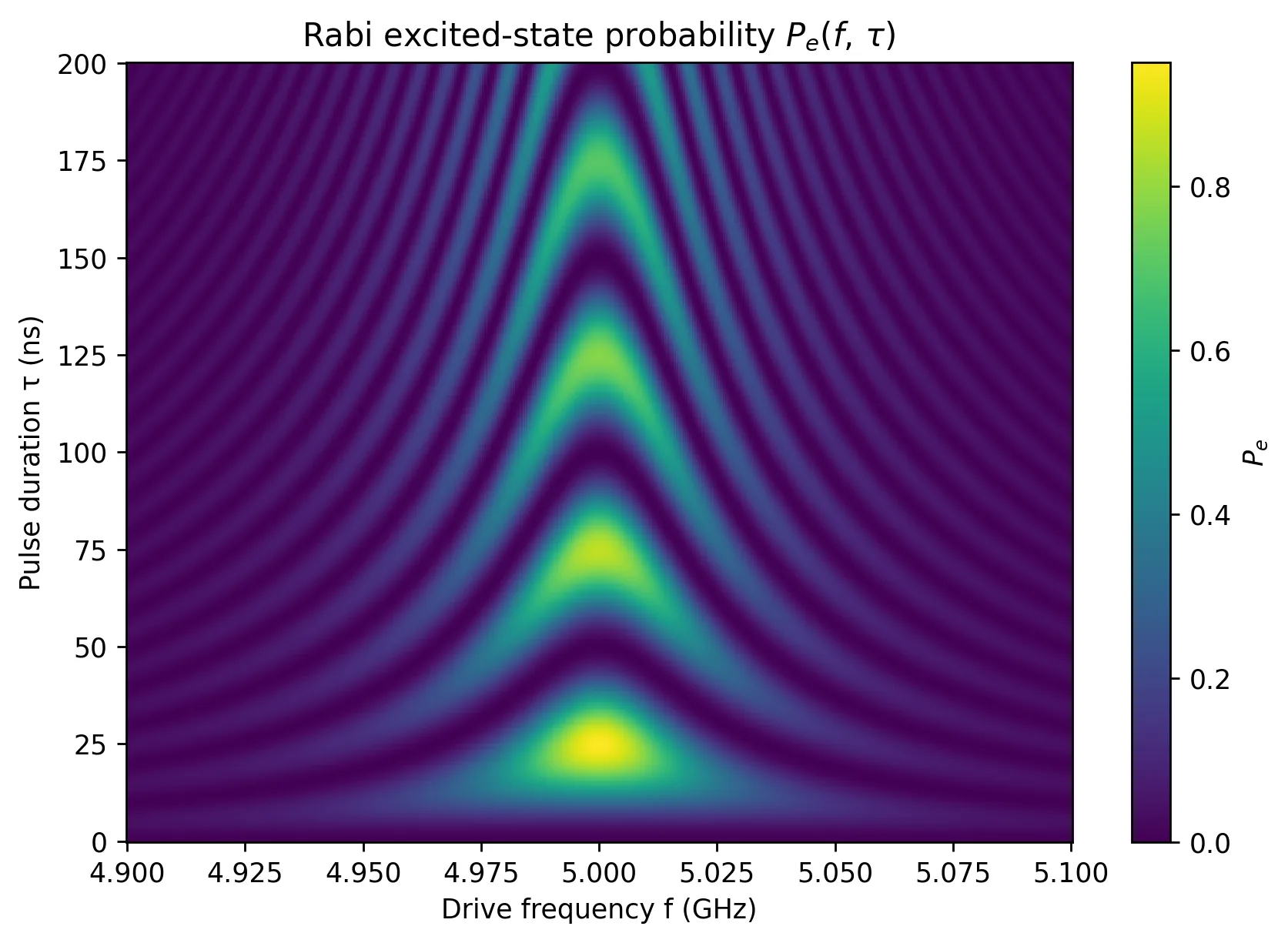
| 7 | Conditional target Rabi (control vs ) | Target oscillation frequency/phase depends on control state due to the term (and any residual ). |
References
- The Quantum Aviary — How the Cross-Resonance Gate Works (overview of , echo, and intuition)
https://thequantumaviary.blogspot.com/2021/07/how-cross-resonance-gate-works.html - Malekakhlagh, Magesan & McKay — First-principles analysis of cross-resonance gate operation, Phys. Rev. A 102, 042605 (2020)
https://link.aps.org/doi/10.1103/PhysRevA.102.042605 - Magesan & Gambetta — Effective Hamiltonian models of the cross-resonance gate, Phys. Rev. A 101, 052308 (2020)
https://link.aps.org/doi/10.1103/PhysRevA.101.052308
#@title Cross-Resonance (CR) gate — slices & heatmaps (PRA 2020 formulas)

from dataclasses import dataclass
from typing import Tuple
import math
import numpy as np
import matplotlib.pyplot as plt

# -----------------------------
# Control knobs (MHz)
# -----------------------------
@dataclass
class CRKnobs:
    f_c: float = 5114.0        # control frequency
    f_t: float = 4914.0        # target frequency
    alpha_c: float = -330.0    # control anharmonicity (negative)
    alpha_t: float = -330.0    # target anharmonicity
    J: float = 3.8             # exchange coupling
    Omega0: float = 30.0       # default drive for Δ-slices
    use_energy_basis: bool = False  # toggle ν-corrections (~10–15%)

    # Sweep grids
    delta_span: Tuple[float, float] = (-500.0, 500.0)
    delta_points: int = 1801
    omega_span: Tuple[float, float] = (0.0, 60.0)
    omega_points: int = 361

K = CRKnobs()

# -----------------------------
# Helpers & ν-coefficients
# -----------------------------
def _safe_div(a: float, b: float, eps: float = 1e-12) -> float:
    """Return a/b with a small guard to avoid blow-ups at poles."""
    if abs(b) < eps:
        return np.sign(b) * 1e12
    return a / b

def _epsilon_from_alpha_over_omega(alpha_mhz: float, omega_mhz: float) -> float:
    """Solve ε from (9 − 4r) ε² + 16(1 − r) ε + 64 r = 0, with r = α/ω."""
    r = alpha_mhz / omega_mhz
    A = (9.0 - 4.0 * r)
    B = 16.0 * (1.0 - r)
    C = 64.0 * r
    disc = max(B * B - 4.0 * A * C, 0.0)
    if abs(A) < 1e-15:
        return 0.2
    e1 = (-B + math.sqrt(disc)) / (2.0 * A)
    e2 = (-B - math.sqrt(disc)) / (2.0 * A)
    roots = [e for e in (e1, e2) if e > 0.0 and np.isfinite(e)]
    return min(roots) if roots else 0.2

def _nu_energy_basis(alpha_mhz: float, omega_mhz: float) -> Tuple[float, float]:
    """Energy-basis ν_01, ν_12 up to O(ε²)."""
    eps = _epsilon_from_alpha_over_omega(alpha_mhz, omega_mhz)
    nu01 = 1.0 - (1.0 / 8.0) * eps - (11.0 / 256.0) * (eps ** 2)
    nu12 = (1.0 - 0.25 * eps - (73.0 / 512.0) * (eps ** 2)) / math.sqrt(2.0)
    return nu01, nu12

def _nu_kerr() -> Tuple[float, float]:
    """Kerr-limit charge matrix elements."""
    return 1.0, 1.0 / math.sqrt(2.0)

if K.use_energy_basis:
    nu_c01, nu_c12 = _nu_energy_basis(K.alpha_c, K.f_c)
    nu_t01, nu_t12 = _nu_energy_basis(K.alpha_t, K.f_t)
else:
    nu_c01, nu_c12 = _nu_kerr()
    nu_t01, nu_t12 = _nu_kerr()

# -----------------------------
# Leading-order rates (MHz)
# -----------------------------
def omega_zx_mhz(delta_ct: float, J: float, Omega: float, alpha_c: float) -> float:
    r"""Entangling rate ω_ZX ≈ JΩ[(Δ+α_c)^{-1} − Δ^{-1}] with small ν-correction."""
    kerr = J * Omega * (_safe_div(1.0, delta_ct + alpha_c) - _safe_div(1.0, delta_ct))
    eb = 0.5 * J * Omega * nu_t01 * (
        (nu_c12 ** 2) * _safe_div(1.0, delta_ct + alpha_c) - 2.0 * (nu_c01 ** 2) * _safe_div(1.0, delta_ct)
    )
    return 0.5 * (kerr + eb)

def omega_zz_mhz(delta_ct: float, J: float, alpha_c: float, alpha_t: float) -> float:
    r"""Static ZZ ≈ J²[(Δ−α_t)^{-1} − (Δ+α_c)^{-1}] with small ν-correction."""
    kerr = (J ** 2) * (_safe_div(1.0, delta_ct - alpha_t) - _safe_div(1.0, delta_ct + alpha_c))
    eb = 0.5 * (J ** 2) * (
        (nu_c01 ** 2) * (nu_t12 ** 2) * _safe_div(1.0, delta_ct - alpha_t) -
        (nu_t01 ** 2) * (nu_c12 ** 2) * _safe_div(1.0, delta_ct + alpha_c)
    )
    return 0.5 * (kerr + eb)

# Region boundaries (poles) for I–V:
REGION_LINES = (K.alpha_t, 0.0, -K.alpha_c / 2.0, -K.alpha_c, -1.5 * K.alpha_c)
def _annotate_regions(ax):
    for x in REGION_LINES:
        ax.axvline(x, linestyle="--", linewidth=1.0)

# -----------------------------
# Slices
# -----------------------------
DELTA = np.linspace(K.delta_span[0], K.delta_span[1], K.delta_points)
OMEGA = np.linspace(K.omega_span[0], K.omega_span[1], K.omega_points)

wzx_slice = np.array([omega_zx_mhz(d, K.J, K.Omega0, K.alpha_c) for d in DELTA])
wzz_slice = np.array([omega_zz_mhz(d, K.J, K.alpha_c, K.alpha_t) for d in DELTA])
ratio_slice = np.abs(np.where(np.abs(wzz_slice) > 1e-12, wzx_slice / wzz_slice, np.nan))

# Plot 1: ω_ZX vs Δ_ct
plt.figure(figsize=(8, 5), dpi=150)
plt.plot(DELTA, wzx_slice, label=rf'$\omega_{{ZX}}$ (Ω={K.Omega0:.1f} MHz)', color='blue')
plt.axhline(0.0, linestyle=":")
_annotate_regions(plt.gca())
plt.xlabel(r'$\Delta_{ct}$ (MHz)')
plt.ylabel(r'$\omega_{ZX}$ (MHz)')
plt.title(r'Leading-order $\omega_{ZX}$ vs detuning')
plt.legend()
plt.show()

# Plot 2: ω_ZZ vs Δ_ct
plt.figure(figsize=(8, 5), dpi=150)
plt.plot(DELTA, wzz_slice, label=r'$\omega_{ZZ}$ (static; lowest order)', color='blue')
plt.axhline(0.0, linestyle=":")
_annotate_regions(plt.gca())
plt.xlabel(r'$\Delta_{ct}$ (MHz)')
plt.ylabel(r'$\omega_{ZZ}$ (MHz)')
plt.title(r'Lowest-order $\omega_{ZZ}$ vs detuning')
plt.legend()
plt.show()

# Heatmap 1: ω_ZX(Δ, Ω)
wzx_map = np.empty((DELTA.size, OMEGA.size))
for i, d in enumerate(DELTA):
    for j, om in enumerate(OMEGA):
        wzx_map[i, j] = omega_zx_mhz(d, K.J, om, K.alpha_c)

plt.figure(figsize=(8, 6), dpi=150)
extent = [OMEGA.min(), OMEGA.max(), DELTA.min(), DELTA.max()]
plt.imshow(wzx_map, origin="lower", aspect="auto", extent=extent, cmap="magma")
plt.colorbar(label=r'$\omega_{ZX}$ (MHz)')
plt.xlabel(r'$\Omega$ (MHz)')
plt.ylabel(r'$\Delta_{ct}$ (MHz)')
plt.title(r'$\omega_{ZX}(\Delta_{ct}, \Omega)$ (leading-order)')
plt.show()

# Heatmap 2: |ω_ZX/ω_ZZ|(Δ, Ω) (clipped for visibility)
ratio_map = np.empty_like(wzx_map)
for i, d in enumerate(DELTA):
    zz = omega_zz_mhz(d, K.J, K.alpha_c, K.alpha_t)
    for j, om in enumerate(OMEGA):
        zx = omega_zx_mhz(d, K.J, om, K.alpha_c)
        ratio_map[i, j] = abs(zx / zz) if abs(zz) > 1e-12 else np.nan

clip_max = np.nanpercentile(ratio_map[np.isfinite(ratio_map)], 99.5)
ratio_map_vis = np.clip(ratio_map, 0.0, clip_max)

plt.figure(figsize=(8, 6), dpi=150)
plt.imshow(ratio_map_vis, origin="lower", aspect="auto", extent=extent)
plt.colorbar(label=r'$|\omega_{ZX}/\omega_{ZZ}|$')
plt.xlabel(r'$\Omega$ (MHz)')
plt.ylabel(r'$\Delta_{ct}$ (MHz)')
plt.title(r'Heuristic $|\omega_{ZX}/\omega_{ZZ}|$ map (clipped at 99.5th pct)')
plt.show()
#@title Echoed-CR demonstration (two-segment echo, Eqs. 28a–d in PRA 2020)

import math
import numpy as np
import matplotlib.pyplot as plt

def omega_echo_coeffs(zx_mhz: float, ix_mhz: float, iz_mhz: float, zz_mhz: float, tau_ns: float):
    """Return (u_ii, u_iy, u_iz, u_zx) after a +Ω / Xπ / −Ω echo; MHz→rad/ns inside."""
    conv = 2.0 * math.pi / 1000.0
    zx, ix, iz, zz = zx_mhz*conv, ix_mhz*conv, iz_mhz*conv, zz_mhz*conv
    w_plus  = math.sqrt((zx + ix)**2 + (iz + zz)**2)
    w_minus = math.sqrt((zx - ix)**2 + (iz - zz)**2)
    c_plus, s_plus = math.cos(0.5*w_plus*tau_ns), math.sin(0.5*w_plus*tau_ns)
    c_minus, s_minus = math.cos(0.5*w_minus*tau_ns), math.sin(0.5*w_minus*tau_ns)
    denom = (w_plus*w_minus + 1e-30)
    u_ii = c_plus*c_minus + ((ix**2 - iz**2 - zx**2 + zz**2)/denom)*s_plus*s_minus
    u_iy = 2j*(zx*zz - ix*iz)/denom * s_plus*s_minus
    u_iz = 1j*((zz - iz)/(w_minus + 1e-30))*c_plus*s_minus - 1j*((zz + iz)/(w_plus + 1e-30))*s_plus*c_minus
    u_zx = 1j*((ix - zx)/(w_minus + 1e-30))*c_plus*s_minus - 1j*((ix + zx)/(w_plus + 1e-30))*s_plus*c_minus
    return u_ii, u_iy, u_iz, u_zx

# Representative point near Region III speed-up:
f_c, f_t = 5114.0, 4914.0
alpha_c = -330.0
J, Omega = 3.8, 30.0
delta0 = f_c - f_t

def omega_zx_mhz(delta_ct, J, Omega, alpha_c):
    return J*Omega*(1.0/(delta_ct + alpha_c) - 1.0/max(delta_ct, 1e-12))

w_zx = omega_zx_mhz(delta0, J, Omega, alpha_c)
w_ix, w_iz, w_zz = 1.0, 10.0, 0.1   # illustrative single-qubit terms / static ZZ
tau_ns = 100.0

u_ii, u_iy, u_iz, u_zx = omega_echo_coeffs(w_zx, w_ix, w_iz, w_zz, tau_ns)

plt.figure(figsize=(7.5, 4.8), dpi=150)
labels = [r'$|u_{ZX}|$', r'$|u_{IY}|$', r'$|u_{IZ}|$']
vals = [abs(u_zx), abs(u_iy), abs(u_iz)]
x = np.arange(len(labels))
plt.bar(x, vals)
plt.xticks(x, labels)
plt.ylabel('Coefficient magnitude (unitless)')
plt.title('Echoed-CR: effective coefficients after two-segment echo')
plt.show()
#@title Conditional target Rabi under CR effective Hamiltonian
# we diagonalize once and propagate.

from dataclasses import dataclass
import math
import numpy as np
import matplotlib.pyplot as plt

# -----------------------------
# Control knobs (MHz unless noted)
# -----------------------------
@dataclass
class RabiKnobs:
    f_c: float = 5114.0          # control frequency
    f_t: float = 4914.0          # target frequency
    alpha_c: float = -330.0      # control anharmonicity
    alpha_t: float = -330.0      # target anharmonicity
    J: float = 3.8               # exchange coupling
    Omega: float = 30.0          # CR drive amplitude on control

    # Residuals (typical orders, tweak for your device)
    wIX_mhz: float = 1.0         # IX (drive crosstalk on target)
    wIZ_khz: float = 20.0        # IZ (AC Stark on target)
    wZI_mhz: float = 10.0        # ZI (AC Stark on control)
    wZZ_khz: float = 100.0       # ZZ (static coupling residual)

    # Time axis
    t_end_ns: float = 400.0
    n_steps: int = 2001

K = RabiKnobs()

# -----------------------------
# Helpers and literature-rate formulas
# -----------------------------
def _safe_div(a: float, b: float, eps: float = 1e-12) -> float:
    return a / (b if abs(b) >= eps else np.sign(b) * eps)

def hz_to_rad_per_ns(hz: float) -> float:
    return 2.0 * math.pi * hz * 1e-9

def mhz_to_rad_per_ns(mhz: float) -> float:
    return hz_to_rad_per_ns(mhz * 1e6)

def khz_to_rad_per_ns(khz: float) -> float:
    return hz_to_rad_per_ns(khz * 1e3)

# Leading-order CR analytics (weak drive, effective model)
# ω_ZX ≈ J Ω [1/(Δ+α_c) − 1/Δ],   ω_ZZ ≈ J^2 [1/(Δ−α_t) − 1/(Δ+α_c)]
def omega_zx_mhz(delta_ct: float, J: float, Omega: float, alpha_c: float) -> float:
    return J * Omega * (_safe_div(1.0, delta_ct + alpha_c) - _safe_div(1.0, delta_ct))

def omega_zz_mhz(delta_ct: float, J: float, alpha_c: float, alpha_t: float) -> float:
    return (J ** 2) * (_safe_div(1.0, delta_ct - alpha_t) - _safe_div(1.0, delta_ct + alpha_c))

# -----------------------------
# Build H_eff (4×4) in rad/ns
# -----------------------------
I2 = np.eye(2)
X = np.array([[0.0, 1.0],
              [1.0, 0.0]])
Z = np.array([[1.0, 0.0],
              [0.0, -1.0]])

def kron2(a, b): return np.kron(a, b)

def build_heff_radns(K: RabiKnobs) -> np.ndarray:
    Δ = K.f_c - K.f_t
    w_zx = mhz_to_rad_per_ns(omega_zx_mhz(Δ, K.J, K.Omega, K.alpha_c))
    w_zz = mhz_to_rad_per_ns(omega_zz_mhz(Δ, K.J, K.alpha_c, K.alpha_t)) + khz_to_rad_per_ns(K.wZZ_khz)
    w_ix = mhz_to_rad_per_ns(K.wIX_mhz)
    w_iz = khz_to_rad_per_ns(K.wIZ_khz)
    w_zi = mhz_to_rad_per_ns(K.wZI_mhz)
    return ((w_ix/2.0) * kron2(I2, X) +
            (w_iz/2.0) * kron2(I2, Z) +
            (w_zi/2.0) * kron2(Z,  I2) +
            (w_zx/2.0) * kron2(Z,  X) +
            (w_zz/2.0) * kron2(Z,  Z))

# -----------------------------
# Time evolution via diagonalization
# -----------------------------
def evolve_state_constH(H: np.ndarray, psi0: np.ndarray, t_ns: np.ndarray) -> np.ndarray:
    E, V = np.linalg.eigh(H)
    Vinv = V.conj().T
    amps0 = Vinv @ psi0
    out = np.empty((psi0.size, t_ns.size), dtype=complex)
    for k, t in enumerate(t_ns):
        out[:, k] = V @ (np.exp(-1j * E * t) * amps0)
    return out

# Basis |00>, |01>, |10>, |11>
e00 = np.array([1,0,0,0], dtype=complex)
e01 = np.array([0,1,0,0], dtype=complex)
e10 = np.array([0,0,1,0], dtype=complex)
e11 = np.array([0,0,0,1], dtype=complex)

# -----------------------------
# Conditional Rabi simulation
# -----------------------------
H = build_heff_radns(K)
t_ns = np.linspace(0.0, K.t_end_ns, K.n_steps)

# Prepare control in |0> (|00>) vs |1> (|10>), target initially |0>
ψ_c0 = evolve_state_constH(H, e00, t_ns)
ψ_c1 = evolve_state_constH(H, e10, t_ns)

# Target |1> probability = P(|01>) + P(|11>)
p_t1_c0 = np.abs(e01.conj() @ ψ_c0)**2 + np.abs(e11.conj() @ ψ_c0)**2
p_t1_c1 = np.abs(e01.conj() @ ψ_c1)**2 + np.abs(e11.conj() @ ψ_c1)**2

# -----------------------------
# Plot
# -----------------------------
plt.figure(figsize=(8.2, 4.8), dpi=150)
plt.plot(t_ns, p_t1_c0, label='Control |0⟩, init |00⟩', color='blue')
plt.plot(t_ns, p_t1_c1, label='Control |1⟩, init |10⟩', color='orange')
plt.xlabel('Time (ns)')
plt.ylabel('Target |1⟩ probability')
plt.title('Conditional target Rabi under CR effective Hamiltonian')
plt.legend()
plt.show()
More expert notes
Browse all expert notes
Stay in the loop.
Get the latest tutorials, demos, and project showcases straight to your inbox. No noise, just the good stuff.
Enable JavaScript to sign up.
Qollab updates only. Unsubscribe any time. Privacy Policy.
On this page