2-qubit states, visualized 8 ways

A 2-qubit state is a four-dimensional complex vector. That's easy to write down and hard to picture, and entanglement makes it harder: the most interesting thing about the state is precisely the part you can't see by looking at each qubit alone. This walkthrough takes one small circuit and renders its state eight different ways, because each visualization makes a different property visible.

Everything below comes from Onri's runnable notebook, shared openly on GitHub. The code and figures are his, republished here with permission. You can run the whole thing end to end in Google Colab.

One circuit, two states

The experiment is a controlled comparison. First, the baseline: the product state |00⟩, where each qubit has its own well-defined state and nothing is correlated. Then the same eight visualizations run again on an entangled state, built with a Hadamard, a CNOT, and a couple of single-qubit rotations:

import numpy as np
from qiskit import QuantumCircuit
from qiskit.quantum_info import Statevector, DensityMatrix

# Create a circuit with 2 qubits
qc = QuantumCircuit(2)
qc.h(0)             # Hadamard on q0
qc.cx(0, 1)         # CNOT with q0 as control, q1 as target
qc.ry(np.pi / 4, 1) # Y-rotation of pi/4 on q1
qc.z(1)             # Phase flip (Z gate) on q1

final_statevector = Statevector(qc)
final_density_matrix = DensityMatrix(qc)

# Generate all 8 plots for the final state
plot_bloch_multivector_viz(final_density_matrix, "Final Entangled State")
plot_q_sphere_viz(final_density_matrix, "Final Entangled State")
plot_steering_ellipsoid(final_density_matrix, "Steering Ellipsoid for Final State")
visualize_schmidt_decomposition(final_statevector, "Schmidt Decomposition for Final State")
explain_toroidal_geometry()
plot_correlation_invariants(final_density_matrix, "Final Entangled State")
plot_wigner_function(final_density_matrix, "Wigner Functions for Final State")
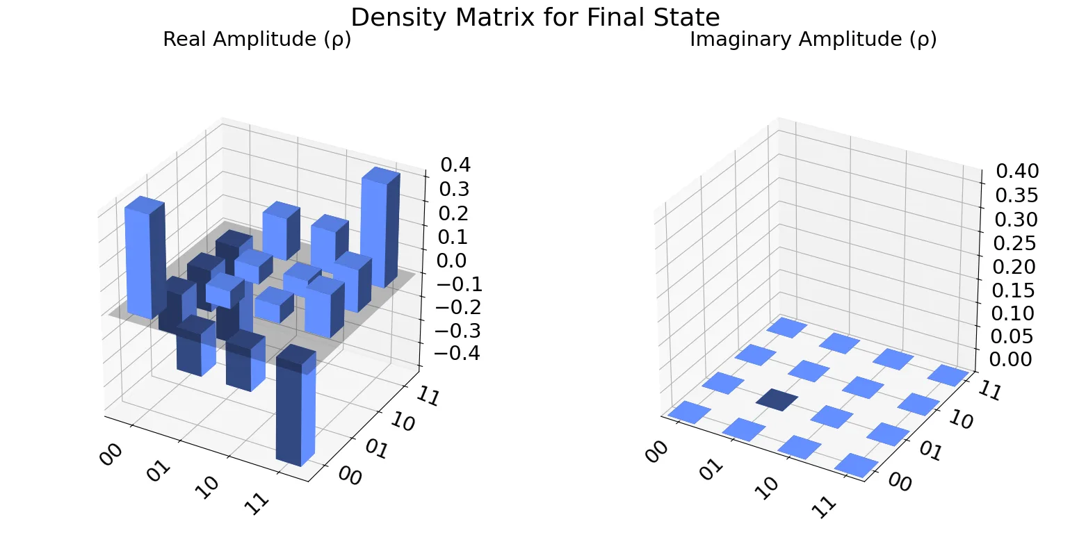
plot_density_matrix(final_density_matrix, "Density Matrix for Final State")

Every method below shows the entangled state; where the contrast with |00⟩ is the whole point, both are shown.

1. Two Bloch spheres, one giveaway

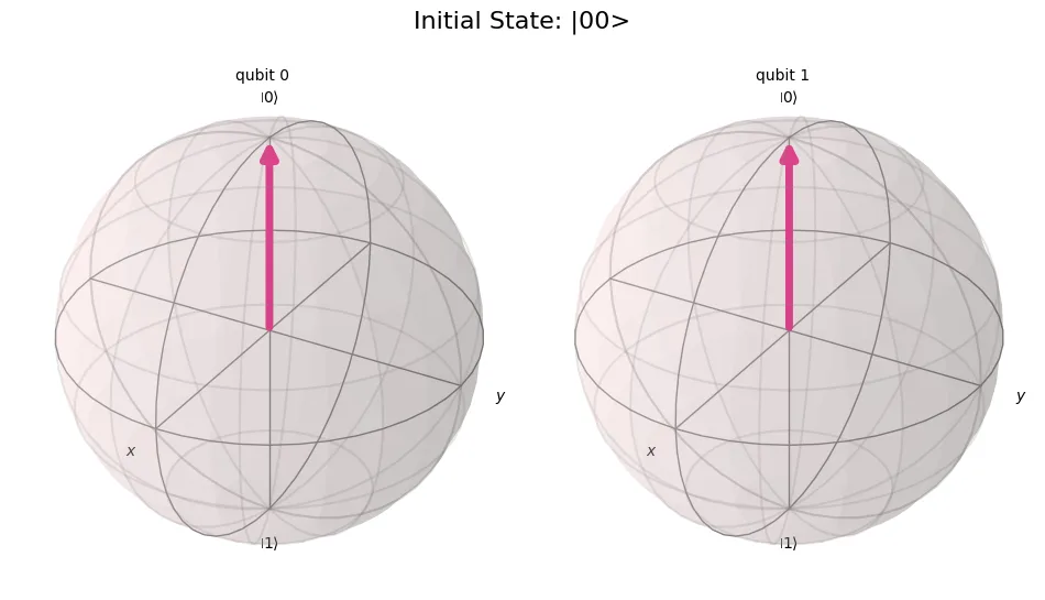
The Bloch multivector shows the state of each qubit on its own Bloch sphere. For |00⟩, both vectors reach the surface: each qubit is in a pure, definite state.

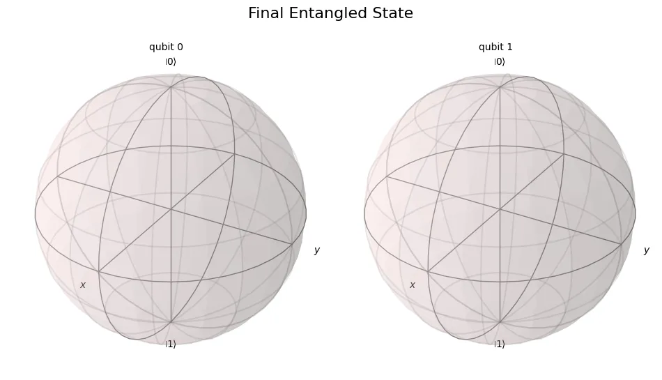
For the entangled state, the vectors retreat inside the sphere. Each qubit on its own looks like a mixed state. The information isn't in either qubit, it's in the correlation between them. The shrunken vector is the visual signature of entanglement.

2. The Q-sphere

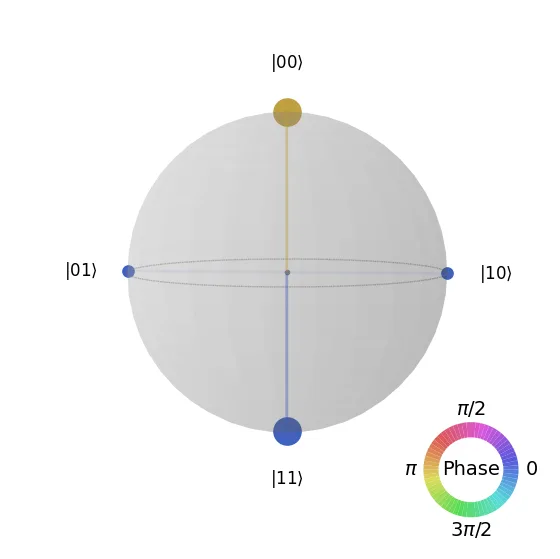
The Q-sphere maps state amplitudes and phases onto a single sphere: the size of each point is the magnitude of the amplitude for a basis state, and its color is the phase. Where the Bloch view loses the correlations, the Q-sphere shows the full 2-qubit state at once.

3. The steering ellipsoid

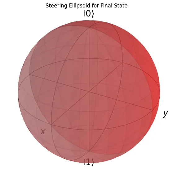
The steering ellipsoid shows the set of states qubit B can be "steered" into by measuring qubit A. If it collapses to a single point, there is no steering at all; a non-trivial ellipsoid means the state is entangled. For |00⟩ the notebook can't even draw one: the ellipsoid degenerates to a point, which is its own kind of answer.

4. Schmidt decomposition

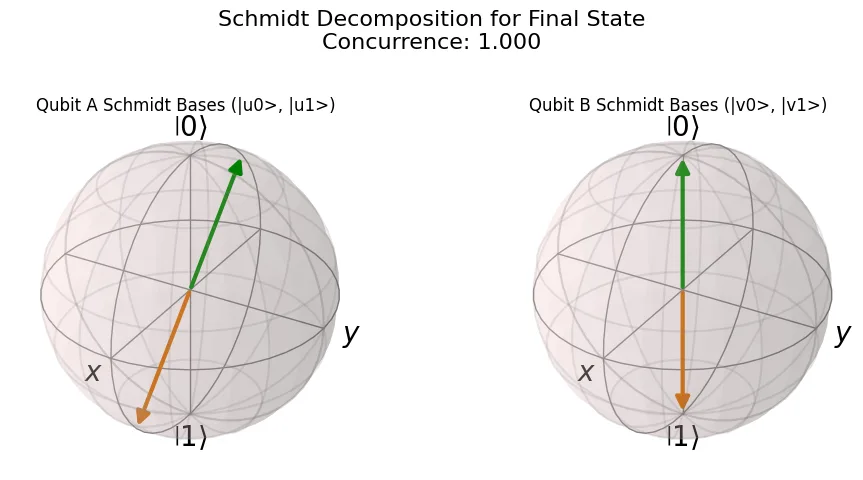
Any pure 2-qubit state can be written as |ψ⟩ = λ₀|u₀⟩|v₀⟩ + λ₁|u₁⟩|v₁⟩. The Schmidt coefficients λ₀ and λ₁ quantify entanglement directly: a product state has one coefficient equal to 1 and the other 0, while an entangled state splits the weight between both terms.

5. Toroidal geometry

Not everything has a standard plot. The toroidal view is a highly abstract method that maps entanglement invariants onto the surface of a torus. Powerful for classifying entanglement, but beyond standard plotting libraries. The notebook explains the concept and moves on; it's included because knowing a representation exists is half of finding a use for it.

6. Correlation invariants

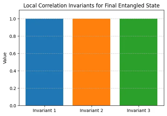
This plot shows the invariants of the state under local unitary operations: the eigenvalues of TᵀT, where T is the correlation matrix. These numbers don't change when either qubit is rotated on its own, so they capture the nature and strength of the correlation itself: the part of the state that no local operation can create or destroy.

7. The Wigner function

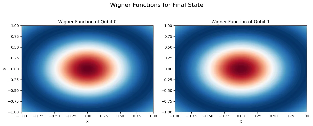
A phase-space representation of each qubit's reduced state. Negative values, shown in red, are a key signature of non-classicality. No classical probability distribution can go below zero.

8. The density matrix

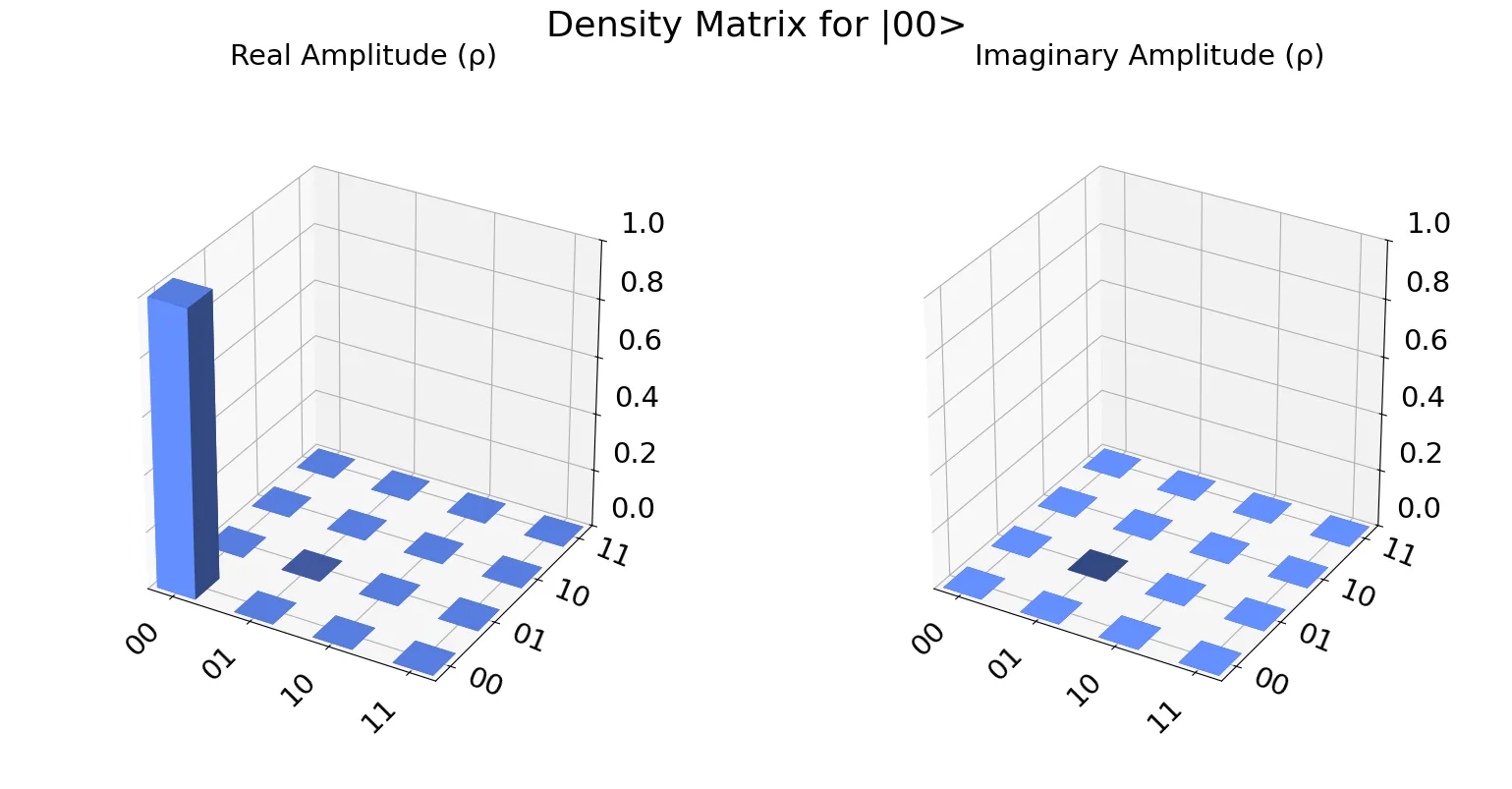
The workhorse. Real parts in blue, imaginary parts in red; the diagonal holds the populations and the off-diagonal elements indicate coherence and entanglement. For |00⟩, a single bar stands alone.

Run it yourself

Every figure above comes out of one script you can run top to bottom: open the notebook on GitHub or run it directly in Colab. Change the circuit in Step 5, run again, and watch all eight views shift together. That's where the intuition comes from.